Information Theory Fundamentals
A complete, single-file reference for the module's information-theory unit: information and entropy, source coding, sources with memory, predictive and run-length coding, channels and mutual information, and channel capacity.
Lectures
Click a lecture to jump to it. Every lecture section has an "↑ Table of Contents" link at its top to jump back here.






Information,
Entropy and the Digital Source
How much information does a message actually carry, and what is the smallest number of bits we truly need in order to send it? This lecture builds the answer from first principles.
- Explain the anatomy of a digital communication system (Tx, channel, Rx) and where information theory fits
- Compute the self-information and entropy of a discrete memoryless source
- Calculate a source’s information rate and explain why fixed-length BCD coding wastes bandwidth
Contents
This page grows as further lectures are added to the document.
1.1 A primer on digital communication systems
The whole module in miniature — transmitter, channel, receiver, and the resources they trade
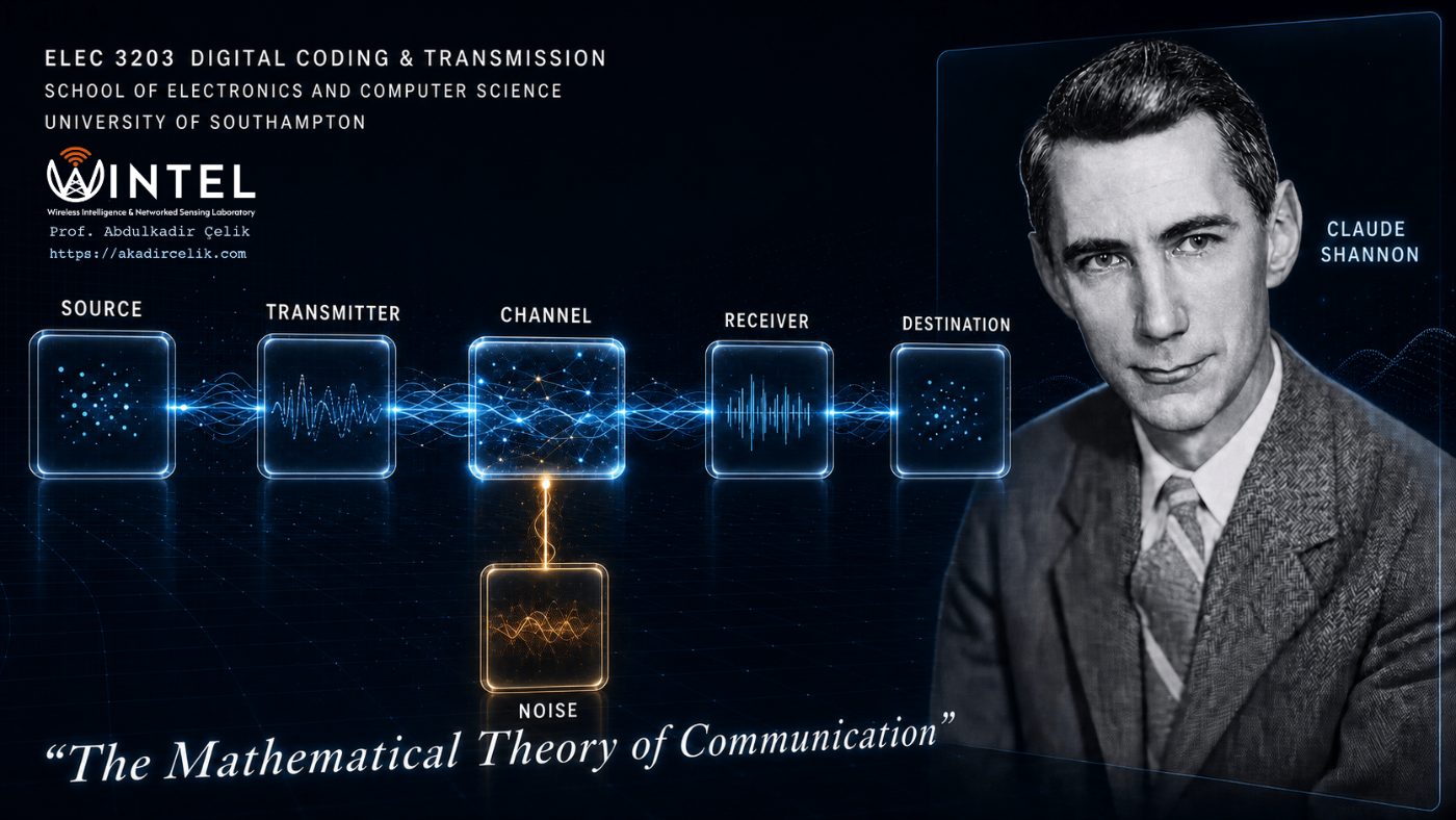
The aim of any telecommunication system is to convey information between two locations that are separated in space, over a channel of adequate quality, at a certain rate and reliably.
This picture is the whole module in miniature. The channel offers a fixed set of resources — transmit power, time, and bandwidth (and, in multi-antenna systems, space) — and the job of the transmitter and receiver design is to spend those resources so as to hit the best possible key performance indicators (KPIs): information rate (how many bits per second get through), latency (how long it takes), reliability (how rarely errors slip past), and energy efficiency (how many bits per joule). Every technique in this module, from source coding to channel coding to modulation, is really a way of trading these resources for these KPIs.
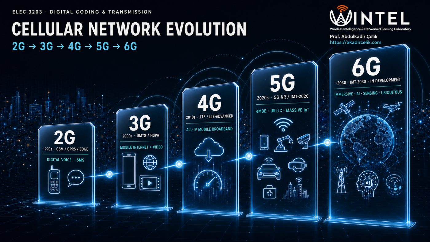
In practice there is no single "best" wireless technology — different applications sit at different points on the resource/KPI trade-off, so the wireless landscape has evolved into a family of standards, each tuned to a different range, data rate, power budget, and device density. Cellular networks (2G–6G) have progressively traded new spectrum and complexity for higher rate, lower latency, and support for ever more connected devices, while short- and medium-range technologies (Bluetooth LE, Zigbee, Wi-Fi, WiMAX, LoRaWAN, NB-IoT) each cover a different rung of the range/power/throughput ladder, from a wrist-worn sensor a few metres away to a smart-city meter kilometres from its gateway.
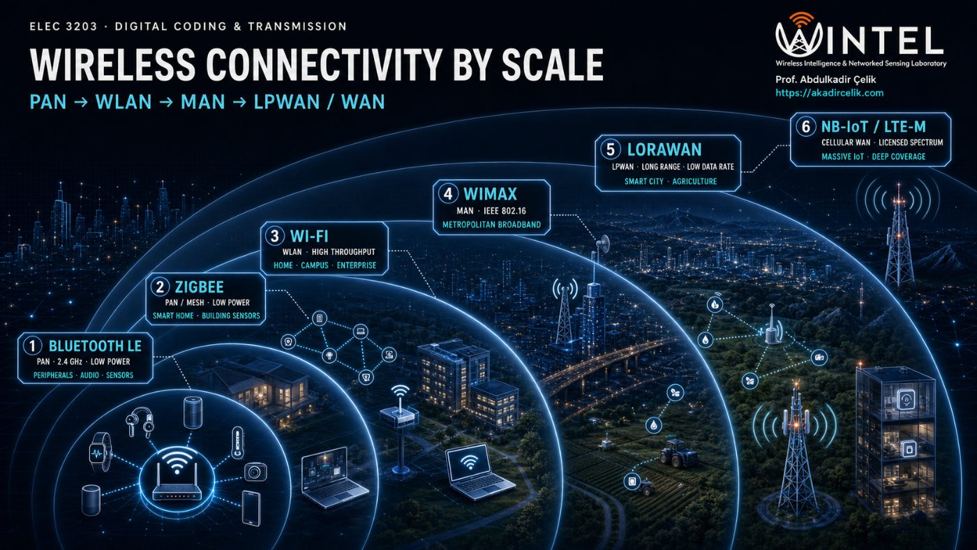
Because the whole module is digital, we first look at how a real source becomes a stream of bits, and then place that stream in the full system.
An analogue source such as speech or video is not digital to begin with. It is turned into a stream of bits by two steps:
With the source reduced to a clean stream of bits, we can place it in the full communication system. A generic digital transmission scheme is a chain of building blocks, with the transmitter along the top, the channel on the right, and the receiver returning along the bottom.
Reading left to right: source coding makes the stream small, channel coding makes it robust, and modulation makes it physical. The receiver simply undoes each step in reverse order.
Treating source coding and channel coding as two separate, independently optimised blocks is convenient and, for a single point-to-point link with an ideal infinite-length code, provably lossless in the limit (Shannon's separation theorem). But real transceivers do not enjoy infinite code length or a fixed, known channel, so joint source-channel coding (JSCC) — designing the two stages together, or replacing them with a single learned mapping from source symbols straight to channel symbols — is increasingly the standard rather than the exception in modern wireless systems, because it can adapt gracefully to unpredictable channel quality where separate coding fails abruptly.
This is also where AI enters the transceiver: deep learning-based JSCC (e.g. autoencoder-style neural encoders/decoders) learns the source-to-channel mapping directly from data, degrading gracefully as channel conditions worsen instead of hitting the "cliff effect" of classical separated designs, and underpins emerging semantic and task-oriented communication schemes being explored for 6G.
This lecture concentrates on the very first block, the source, and asks the most basic question of the whole field. What is information, and how do we measure it?
If the information rate of a source does not exceed the capacity of a channel, then there exists a coding scheme that transmits the information over that channel with an arbitrarily small probability of error, despite the noise. If the rate exceeds capacity, no coding scheme can save you. The whole theorem compresses into one inequality relating the source's information rate \(R\) to the channel's capacity \(C\):
This is an existence result. It promises that a code exists once \(R \le C\), but it does not tell us how to build one, and it says nothing about delay or complexity. Reaching capacity in practice took until the 1990s, when turbo codes appeared. We define \(C\) precisely in Lecture 6, where for a channel of bandwidth \(B\) and signal to noise ratio \(S/N\) it takes the celebrated Shannon and Hartley form \(C = B\log_2(1+S/N)\). For now, Lecture 1 lays the groundwork on the left-hand side of the inequality by measuring the information rate \(R\) that a source produces.
1.2 What is information?
Surprise as a measurable quantity
Consider a weather forecast of rain tomorrow in three places:
The same three words, "it will rain", carry wildly different amounts of information. The rainforest forecast tells us almost nothing, because we knew it already. The desert forecast is a genuine shock. This is the central intuition: information is tied to uncertainty. The more unexpected an event is, meaning the smaller its probability, the more information its occurrence conveys. That single idea is the seed of the entire theory.
A generic digital source is described by four physical quantities:
1.3 Information content of a symbol
Three requirements pin down the function
We want a function \(I(m_i)\) of a symbol's probability \(p_i\) that behaves the way our intuition demands. Three requirements pin it down:
- Monotone in surprise: A smaller \(p_i\) should give a larger \(I\).
- Certainty carries nothing: We need \(I = 0\) when \(p_i = 1\).
- Additive for independent events: Two independent symbols occurring together, with probability \(p_i p_j\), should carry information \(I(m_i) + I(m_j)\). (A short proof that only the logarithm can satisfy this is given in the appendix.)
The additivity requirement is the decisive one. We need \(I(p_i p_j) = I(p_i) + I(p_j)\), that is, a function that turns products into sums. That is exactly the defining property of the logarithm, so \(I(p) \propto \log(1/p)\). Choosing base 2 fixes the unit as the bit:
This measure of information comes from Claude Shannon's 1948 paper "A Mathematical Theory of Communication," written at Bell Labs. Shannon considered several possible bases for the logarithm and chose base 2 because it matches the natural unit of a digital system, the binary digit. He credited the term "bit" itself to his colleague John Tukey, as a contraction of "binary digit." Base
The properties follow immediately from the graph of \(-\log_2 p\):
- Since \(0 \le p_i \le 1\), we have \(I(m_i) \ge 0\), so information is never negative.
- If \(p_i > p_j\), then \(I(m_i) < I(m_j)\), so rarer symbols carry more.
- \(I(m_i) \to 0\) as \(p_i \to 1\), so a certain symbol carries no information.
- \(I(m_i) \to \infty\) as \(p_i \to 0\), so a vanishingly rare symbol carries unbounded information, although it almost never occurs.
1.3.1 Physical interpretation: bits as binary digits
Why "bits"? Because the information content of a symbol equals the smallest number of binary digits needed to label it, in the case where symbols are equally likely:
- 2 equally likely symbols \(\{0,1\}\): one binary digit each, and \(I = \log_2 2 = 1\) bit. ✓
- 4 equally likely symbols \(\{00,01,10,11\}\): two digits each, and \(I = \log_2 4 = 2\) bits. ✓
- \(q\) equally likely symbols: \(\log_2 q\) digits each, and \(I = \log_2 q\) bits. ✓
Assigning \(\log_2 q\) bits to every symbol is called Binary Coded Decimal (BCD). It is exactly right when symbols are equally likely. When they are not, it wastes bits, and fixing that waste is what the rest of Lectures 1 to 4 are about.
1.4 Entropy
Average information per symbol
A single symbol's information varies from one symbol to the next. What matters for system design is the average. Take a long sequence of \(N\) symbols from a memoryless source. Because the symbols are independent and \(N\) is large, symbol \(m_i\) appears about \(p_i N\) times.
Information from symbol \(m_i\) across the whole sequence. It occurs \(p_i N\) times, each occurrence worth \(I(m_i)\):
Total information in the sequence, summed over the alphabet:
Average information per symbol. Divide by \(N\), and \(N\) cancels. This average is the entropy \(H\):
Entropy is a fundamental physical property of the source. It depends only on the alphabet and the probabilities, that is on quantities 1, 2 and 4, and not on the symbol rate. It answers a clear question: on average, how many bits of genuine information does each symbol carry?
A symbol with \(p_i = 0\) never occurs, so it should contribute nothing to the average. Formally \(\lim_{p\to 0^+} p\log_2 p = 0\), so we define \(0\log_2 0 = 0\). This keeps \(H\) well behaved at the edges.
Everything above uses \(\log_2\), giving entropy in bits. Some derivations, including Problem 1.3 below, are easier in natural logarithms. The three common choices are related by a fixed scale factor:
In words: work in whichever base is algebraically convenient, then divide by \(\ln 2 \approx 0.693\) to convert nats back to bits. Base 10 gives a third unit, the hartley, used occasionally in older texts. All three describe the same physical quantity; only the ruler changes.
1.4.1 The binary source and maximum entropy
For a binary source with \(P(1)=p\) and \(P(0)=1-p\), the entropy is the binary entropy function:
Its shape is worth memorising. It is zero at both ends, because a biased coin that almost always lands the same way is predictable and so carries almost no information. It reaches a single maximum of exactly 1 bit at \(p = 0.5\), the fair coin, which is the point of greatest uncertainty.
This generalises. For a \(q\)-ary source, entropy is greatest when all symbols are equally likely, so \(p_i = 1/q\) and \(H_{\max} = \log_2 q\). This gives the key bound, which we revisit throughout the module:
1.5 Information rate
From bits per symbol to bits per second
Entropy is measured per symbol. Multiply it by the symbol rate \(R_s\) to find how many bits of real information the source produces per second. This is the information rate:
Unlike entropy, the information rate depends on all four source quantities, because it includes \(R_s\). It is the true, irreducible demand of the source in bits per second, and it is the target that any good encoder tries to hit.
1.6 Why BCD wastes bandwidth
Sending more bits than you need
If we simply encode every symbol with \(\log_2 q\) bits, which is BCD, the source's output bit rate is:
Since \(H \le \log_2 q\), it follows at once that
So the number of bits we actually send, \(R_b\), is generally larger than the number we truly need to send, \(R\). The gap \(R_b - R\) is pure waste. It matters because, as later lectures show, transmitting at \(R_b\) bits per second costs real resources, namely bandwidth and power. Squeezing \(R_b\) down toward \(R\) is the whole business of efficient source coding, the subject of Lecture 2, which covers Shannon and Fano coding and Huffman coding.
We measure how close a code comes to the ideal by its efficiency \(\eta = H / \bar{L}\), where \(\bar{L}\) is the average codeword length in bits per symbol. BCD gives \(\bar{L} = \log_2 q\), so \(\eta = H/\log_2 q \le 1\). The perfect entropy code reaches \(\eta = 1\), where \(\bar{L} = H\).
Worked examples
MATLAB corner
Three short scripts make the ideas concrete: a reusable entropy function, a plot of the binary entropy curve so you can see the peak at \(p = 0.5\) for yourself, and a real-data check using English letter frequencies.
Problems with solutions
Work each one before reading the solution.
Summary and key formulas
- Information measures surprise. Rarer symbols carry more, and the unit is the bit.
- Entropy is the average information per symbol, a fundamental property of the source that does not depend on the symbol rate.
- Information rate \(R = R_sH\) is the true number of bits per second the source must send.
- BCD spends \(\log_2 q\) bits per symbol and is optimal only for equally likely sources. In general \(R_b \ge R\), which leaves room for efficient coding.
- Next, in Lecture 2: maximum entropy, and building efficient codes with the Shannon and Fano method and Huffman coding, which push \(\bar L\) down toward \(H\).
Appendix: why the logarithm?
Section 3 asked for a function \(I(p)\) with three properties: it decreases as \(p\) increases, it vanishes at \(p=1\), and it is additive, \(I(p_ip_j) = I(p_i) + I(p_j)\), for independent events. Here we show the additivity condition alone, together with the mildest smoothness assumption, forces \(I\) to be a constant multiple of \(\log(1/p)\).
Step 1. Restate additivity as a functional equation. Write \(f(p) = I(p)\) for \(p \in (0,1]\). The requirement is
Step 2. Substitute \(x = y\). Then \(f(x^2) = 2f(x)\), and by induction \(f(x^n) = nf(x)\) for every positive integer \(n\). Applying this with \(x\) replaced by \(x^{1/n}\) gives \(f(x) = n f(x^{1/n})\), so also \(f(x^{m/n}) = \tfrac{m}{n} f(x)\) for positive integers \(m, n\). So \(f(x^r) = r f(x)\) for every positive rational \(r\), and by continuity (our smoothness assumption) for every real \(r > 0\).
Step 3. Fix a reference point. Pick any \(x_0 \in (0,1)\) and define the constant \(c = f(x_0)/\ln(1/x_0) > 0\) (positive because \(f\) decreases and \(\ln(1/x_0) > 0\)). For any other \(p \in (0,1)\) write \(p = x_0^r\) for \(r = \ln p / \ln x_0\). Then by Step 2:
Step 4. Conclude. So \(f(p) = c\ln(1/p)\) for some positive constant \(c\), that is, \(I(p)\) must be a constant multiple of a logarithm of \(1/p\), in any base. Choosing \(c = 1/\ln 2\) turns the constant into \(\log_2\) and fixes the unit as the bit:
No other family of functions, polynomial, exponential, or otherwise, satisfies the additivity requirement. The logarithm is not a convenient modelling choice; it is the only function the axioms allow.
Efficient Source Coding: Shannon-Fano and Huffman
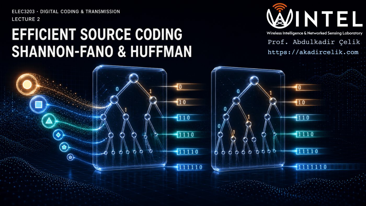
BCD wastes bits whenever symbols are not equally likely. This lecture builds two concrete codes, Shannon-Fano and Huffman, that assign short codewords to common symbols and long ones to rare symbols, pushing the average length down to nearly the entropy bound.
- Construct Shannon-Fano and Huffman codes for a given symbol alphabet
- Compute average codeword length and coding efficiency against the entropy bound
- Explain why Huffman coding is optimal among prefix codes
Contents
This page grows as further lectures are added to the document.
2.1 Maximum entropy: q-ary and binary sources
Where does \(H \le \log_2 q\) come from?
Lecture 1 stated, and proved in its appendix, that the entropy of a \(q\)-ary source is bounded by \(H \le \log_2 q\), with equality only for equiprobable symbols. Here we derive that result directly, by maximising \(H\) subject to the one constraint every probability distribution must satisfy: \(\sum_i p_i = 1\).
2.1.1 Lagrangian derivation for a q-ary source
Suppose you want to maximise (or minimise) some function, but the variables are not free: they must also satisfy a constraint. Here we want to maximise entropy \(H(p_1,\ldots,p_q)\), but the \(p_i\) cannot be chosen independently — they must always sum to 1. Without the constraint, "maximise \(H\)" would have a silly answer (push some \(p_i\) to absurd values), so we need a way to search only among the probability vectors that are actually valid.
The Lagrangian is a trick for turning a constrained problem into an unconstrained one. We build a new function \(\mathcal{L}\) by taking the objective (\(H\)) and adding a penalty term for violating the constraint, weighted by a new variable \(\lambda\) (the Lagrange multiplier):
Notice that whenever the constraint \(\sum_i p_i = 1\) actually holds, the penalty term is exactly zero, so \(\mathcal{L} = H\) at any valid point. This means: any point that maximises \(\mathcal{L}\) while also satisfying the constraint automatically maximises \(H\) too. We have replaced "maximise \(H\) subject to a constraint" with "find a stationary point of \(\mathcal{L}\)", which is a completely ordinary calculus problem with no constraint left to worry about.
Why does setting a derivative to zero find a maximum? This is the basic first-order condition from single-variable calculus, just applied one variable at a time: at the very top of a smooth hill, the slope is momentarily flat — the function is neither increasing nor decreasing in any direction. So at a maximum, the partial derivative with respect to every variable (each \(p_i\), and also \(\lambda\)) must independently equal zero. That gives us one equation per variable, and solving all of them together pins down the maximising point exactly. (This condition alone finds any flat point — a peak, a valley, or a saddle; here we know from the shape of entropy, concave and zero at the boundaries, that the one flat interior point we find must be the maximum.)
This machinery, "Lagrange multipliers", is the standard tool in optimisation for handling equality constraints, and it reappears constantly in engineering (power allocation, resource budgets, rate-distortion problems). The mechanical recipe is always the same three steps: (1) form \(\mathcal{L}\) = objective + \(\lambda\)×(constraint written as "\(= 0\)"), (2) set every partial derivative of \(\mathcal{L}\) to zero, (3) solve the resulting system.
We want to maximise \(H = -\sum_{i=1}^q p_i\log_2 p_i\) subject to \(\sum_{i=1}^q p_i = 1\). Introduce a Lagrange multiplier \(\lambda\) and form the Lagrangian:
Differentiate with respect to a single \(p_i\), remembering \(\dfrac{d}{dx}(x\log_2 x) = \log_2 x + \log_2 e\):
The right-hand side does not depend on \(i\) at all, so every \(p_i\) satisfies the same equation, meaning every \(p_i\) must be equal to the same constant \(c\). Applying the constraint \(\sum_i p_i = 1\) with \(p_i = c\) for all \(i\):
So the entropy of a \(q\)-ary source is maximised exactly when every symbol is equally likely, \(p_i = 1/q\), which (as we already know) gives \(H_{\max} = \log_2 q\). This is the same conclusion as Lecture 1's Problem 2.3, reached this time via calculus rather than an inequality.
2.1.2 The binary case, revisited
Specialising to \(q=2\) with \(p_1 = p\) and \(p_2 = 1-p\) recovers the binary entropy function from Lecture 1, \(H(p) = -p\log_2 p - (1-p)\log_2(1-p)\), maximised at \(p=0.5\) with \(H_{\max}=1\) bit. The figure below is the same curve as Lecture 1, included again here because the whole of this lecture is about closing the gap between \(H\) and \(\log_2 q\).
2.2 Efficient source coding
Coding efficiency and the design rule
We restrict attention to lossless source coding: converting symbols into codewords without throwing away any information, so the original symbols can always be recovered exactly. From Lecture 1, the information rate is
so in general BCD, which always spends \(\log_2 q\) bits per symbol, is not efficient. Coding efficiency compares the information the source truly produces with the rate the code actually uses:
Shannon's source coding theorem guarantees that efficient coding can push this arbitrarily close to 100%: for any memoryless source, there exists a code whose average length \(\bar L\) is as close to \(H\) as we like (exactly \(H\) when all self-informations happen to be integers, and within one bit of \(H\) in general, closer still if we code blocks of symbols together). This lecture builds two such codes, Shannon-Fano and Huffman.
2.2.1 The core idea: match codeword length to information content
When symbols are equiprobable, \(p_i = 1/q\), entropy is already maximal, \(H = \log_2 q\), and coding every symbol with \(\log_2 q\) bits (BCD) achieves \(\text{CE} = 100\%\) automatically. The trouble is only when symbols are not equiprobable: then \(H < \log_2 q\) and BCD is wasteful. The fix follows directly from Lecture 1's definition of information content, \(I(m_i) = -\log_2 p_i\):
Design rule. Assign each symbol a codeword whose length \(\ell_i\) is as close as possible to its own information content \(I(m_i) = -\log_2 p_i\): common symbols get short codewords, rare symbols get long ones. Two practical constraints bind this ideal: codeword lengths must be whole numbers of bits, and no codeword may be a prefix of another, so a decoder can tell where one codeword ends and the next begins just by reading bits left to right.
2.3 Shannon-Fano coding
Split the sorted list from the top down
Shannon-Fano coding builds a variable-length prefix code by repeatedly splitting the symbol list into two halves of roughly equal total probability.
2.3.1 Worked example: eight symbols
Take the same eight symbols as Example 2.1, with \(p = (0.27, 0.20, 0.17, 0.16, 0.06, 0.06, 0.04, 0.04)\), already sorted in descending order. Splitting repeatedly to keep each half's probability mass as equal as possible gives:
| Symbol | \(p_i\) | \(I_i \approx\) (bits) | Step 1 | Step 2 | Step 3 | Step 4 | Codeword |
|---|---|---|---|---|---|---|---|
| m₁ | 0.27 | 1.89 | 0 | 0 | 00 | ||
| m₂ | 0.20 | 2.32 | 0 | 1 | 01 | ||
| m₃ | 0.17 | 2.56 | 1 | 0 | 0 | 100 | |
| m₄ | 0.16 | 2.64 | 1 | 0 | 1 | 101 | |
| m₅ | 0.06 | 4.06 | 1 | 1 | 0 | 0 | 1100 |
| m₆ | 0.06 | 4.06 | 1 | 1 | 0 | 1 | 1101 |
| m₇ | 0.04 | 4.64 | 1 | 1 | 1 | 0 | 1110 |
| m₈ | 0.04 | 4.64 | 1 | 1 | 1 | 1 | 1111 |
Notice the pattern: the two most probable symbols get 2-bit codewords, the middle two get 3 bits, and the four rarest share 4 bits each, tracking their information content \(I_i\) closely.
Grouping by codeword length, \(0.27+0.20=0.47\) of the mass uses 2 bits, \(0.17+0.16=0.33\) uses 3 bits, and \(0.06+0.06+0.04+0.04=0.20\) uses 4 bits. The average codeword length is:
With \(H = 2.6906\) bits/symbol from Example 2.1, the coding efficiency is:
Compare this with the 89.69% of fixed 3-bit codewords on the very same symbols: variable-length coding recovers almost all of the wasted 10.31 percentage points, using only whole numbers of bits per symbol.
2.3.2 A cleaner example: powers-of-two probabilities
Shannon-Fano reaches exactly 100% efficiency whenever every probability is a negative power of two, because then each split can be made perfectly even. Take eight symbols with \(p = (\tfrac12, \tfrac14, \tfrac18, \tfrac1{16}, \tfrac1{32}, \tfrac1{64}, \tfrac1{128}, \tfrac1{128})\):
| Symbol \(X_i\) | Prob. \(P(X_i)\) | \(I\) (bits) | Codeword | bits/symbol | ||||||
|---|---|---|---|---|---|---|---|---|---|---|
| 1 | 2 | 3 | 4 | 5 | 6 | 7 | ||||
| A | \(\frac{1}{2}\) | 1 | 0 | 1 | ||||||
| B | \(\frac{1}{4}\) | 2 | 1 | 0 | 2 | |||||
| C | \(\frac{1}{8}\) | 3 | 1 | 1 | 0 | 3 | ||||
| D | \(\frac{1}{16}\) | 4 | 1 | 1 | 1 | 0 | 4 | |||
| E | \(\frac{1}{32}\) | 5 | 1 | 1 | 1 | 1 | 0 | 5 | ||
| F | \(\frac{1}{64}\) | 6 | 1 | 1 | 1 | 1 | 1 | 0 | 6 | |
| G | \(\frac{1}{128}\) | 7 | 1 | 1 | 1 | 1 | 1 | 1 | 0 | 7 |
| H | \(\frac{1}{128}\) | 7 | 1 | 1 | 1 | 1 | 1 | 1 | 1 | 7 |
Here every codeword length exactly equals its symbol's information content, so \(H = \bar L\) precisely:
giving \(\text{CE} = 100\%\). By contrast, a fixed 3-bit code for these 8 symbols (needed because \(\lceil\log_2 8\rceil = 3\)) would give only \(\text{CE} = 1.984/3 = 66\%\). This is the cleanest possible illustration of the design rule from Section 2.1: match codeword length to information content, exactly, whenever the probabilities allow it.
2.4 Huffman coding
Merge the least probable items from the bottom up
Huffman coding builds the same kind of variable-length prefix code as Shannon-Fano, but from the bottom up instead of the top down: it repeatedly merges the two least probable symbols into a combined subgroup, rather than repeatedly splitting the whole list in two.
2.4.1 Worked example: the same eight symbols
Apply Huffman coding to the same alphabet as Section 3.1, \(p = (0.27, 0.20, 0.17, 0.16, 0.06, 0.06, 0.04, 0.04)\), so the two methods can be compared directly. Building the tree takes 7 merges (one per internal node); each step below shows the currently active items sorted by probability and the two least probable highlighted for merging, and the new combined item that carries into the next step.
The same construction is often easier to read as an actual tree: the root splits repeatedly until every leaf is a single symbol, and a symbol's codeword is just the string of 0s and 1s collected root-to-leaf.
Reading a symbol's codeword means walking from the root down to its leaf and recording each 0/1 along the way, then reading that path bottom-up (root-first) is exactly the order the bits are transmitted in — for example m₅ sits inside m₅₆₇₈(bit 1 at the root) → m₅₆₇₈(bit 1) → m₅₆(bit 0) → m₅(bit 0), giving codeword 1100, exactly matching the table below.
Reading each symbol's path from the root, then reversing the bit order, gives the codewords:
| Symbol | \(p_i\) | Codeword | bits |
|---|---|---|---|
| m₁ | 0.27 | 01 | 2 |
| m₂ | 0.20 | 10 | 2 |
| m₃ | 0.17 | 000 | 3 |
| m₄ | 0.16 | 001 | 3 |
| m₅ | 0.06 | 1100 | 4 |
| m₆ | 0.06 | 1101 | 4 |
| m₇ | 0.04 | 1110 | 4 |
| m₈ | 0.04 | 1111 | 4 |
The length distribution is identical to Shannon-Fano's for this example (two 2-bit, two 3-bit, four 4-bit codewords), so:
The two methods reach the same efficiency here, though in general their individual codeword assignments (which symbol gets which specific bit string) can differ, even when the length distribution matches.
2.5 Comparing the two methods
Greedy split versus provable optimum
- Both belong to the class of entropy coding methods: they assign codeword length as close as possible to each symbol's information content.
- Both produce prefix codes, so the encoded bit stream can always be decoded unambiguously.
- For an alphabet of \(q\) symbols, the longest codeword in either scheme can be as long as \(q-1\) bits, which becomes impractical (large decoding buffers, high latency) for large alphabets.
- Huffman coding is provably optimal (minimum \(\bar L\) among prefix codes); Shannon-Fano is usually close but not guaranteed optimal. In practice the coding efficiency of the two is nearly identical, as both worked examples above show.
MATLAB corner
MATLAB's Communications Toolbox ships huffmandict and huffmanenco/huffmandeco, but writing the design rule out by hand builds real intuition. The script below builds a Huffman code from scratch and checks it against Example 2.1's numbers.
Problems with solutions
Work each one before revealing the solution.
Summary and key formulas
- Maximum entropy occurs at equiprobable symbols, \(H_{\max} = \log_2 q\), proved here by Lagrange multipliers.
- Efficient coding assigns codeword length close to each symbol's information content; BCD only does this when symbols are already equiprobable.
- Shannon-Fano splits the sorted symbol list top-down to balance probability mass at each step.
- Huffman merges the least-probable symbols bottom-up, and is provably optimal among prefix codes.
- Both are prefix codes, decodable unambiguously, and both push coding efficiency close to 100% wherever the underlying probabilities allow it.
- Next, in Lecture 3: sources with memory, where correlation between symbols opens up further gains beyond what a memoryless entropy code can achieve.
Sources with Memory: Markov Models
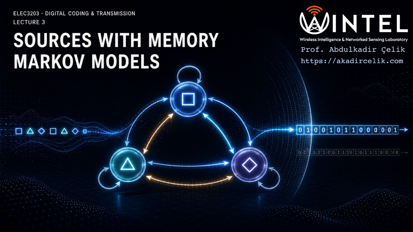
Lectures 1 and 2 assumed a memoryless source: each symbol independent of the last. Real sources, speech, images, text, are correlated. This lecture models that correlation with Markov chains, shows why it lowers entropy below the memoryless bound, and explains why coding a memory source as if it were memoryless wastes bits.
- Model a source with memory as a discrete Markov chain and derive its state probabilities
- Compute the entropy of a Markov source and compare it with the memoryless bound
- Explain why exploiting symbol dependence reduces the achievable code rate
Contents
This page grows as further lectures are added to the document.
3.1 Redundancy in real-world sources
Real signals are not memoryless
Every source in Lectures 1 and 2 was memoryless: each emitted symbol was statistically independent of every other. That assumption made the maths tractable, but it is rarely true of real signals. Speech, images, and text all exhibit correlation between neighbouring samples or symbols — a sampled speech waveform changes slowly relative to the sampling rate, so consecutive samples tend to sit close together, and English text has strong letter- and word-level correlations ("q" is almost always followed by "u").
This correlation is a form of redundancy: knowing the recent past lets you narrow down, sometimes drastically, what symbol comes next. Given a source that has just emitted a run of large positive speech samples, the next sample is very unlikely to be a large negative one. Redundancy of this kind should be exploited during coding, because a symbol that is largely predictable from its neighbours carries very little new information.
The practical consequence is important: applying an entropy code (Shannon-Fano, Huffman) designed for a memoryless source directly to a correlated sequence, as if each symbol were independent, throws away the redundancy between symbols and leaves real compression gains on the table. This lecture makes that statement precise.
3.2 Modelling memory: Markov processes
A bounded window of the past, not the entire history
To reason about correlated sources quantitatively we need a model of the dependency, not just a qualitative sense that "nearby symbols are related". The standard model is a Markov process: a source emitting symbols \(\{S(k)\}\) indexed by discrete time \(k\), in which the current symbol depends on a bounded window of past symbols rather than the entire history.
- First-order Markov process: the current symbol depends only on the immediately preceding one, \(P\big(S(k)\mid S(k-1)\big)\).
- \(N\)th-order Markov process: the current symbol depends on the \(N\) preceding symbols, \(P\big(S(k)\mid S(k-1),\ldots,S(k-N)\big)\).
First-order chains are by far the most widely used, since higher orders quickly become unwieldy: a \(q\)-symbol alphabet needs a \(q\times q\) transition matrix at order 1, but \(q^{N+1}\) transition probabilities at order \(N\). For a modest 8-symbol alphabet the parameter count explodes within a few orders:
3.2.1 The two-state first-order Markov source
The simplest non-trivial case has just two states, \(X_1\) and \(X_2\) (equivalently, symbols "1" and "2"). Being in a state and then moving to the next symbol is governed by four transition probabilities, arranged in the matrix \(\Gamma\):
The prior probabilities \(P_1=P(X_1)\) and \(P_2=P(X_2)\) describe how often the source sits in each state overall (i.e. \(P(S(0){=}1)=P_1\)); the transition probabilities \(p_{ij}=P(S(k){=}j\mid S(k-1){=}i)\) describe how the source moves between states from one symbol to the next.
3.2.2 Predictive models: an equivalent view
An alternative, and closely related, way to model memory is a predictive model. If \(S(k)\) is influenced by its \(N\) predecessors, write
where \(f(\cdot)\) is a prediction built from the recent past, and \(\varepsilon(k)\), the innovation, is whatever about \(S(k)\) could not be predicted from those past values. A common special case is the \(N\)th-order linear autoregressive (AR) model, \(S(k)=\sum_{j=1}^{N} a_j S(k-j) + \varepsilon(k)\), widely used for speech.
The goal of a good predictive model is to make \(\{\varepsilon(k)\}\) nearly uncorrelated and zero-mean, so that almost all of the redundancy in \(\{S(k)\}\) has been absorbed into the prediction \(f(\cdot)\), and only the small, near-independent innovation remains to be coded. We return to this idea in Section 5 and pick it up properly as source coding for memory sources in the next lecture.
3.2.3 Model order versus complexity
First-order Markov chains are by far the most common model in practice, for a concrete reason: a \(q\)-symbol alphabet needs only a \(q\times q\) transition matrix at order 1, but a full \(N\)th-order model needs \(q^{N+1}\) transition probabilities — the table grows exponentially with the memory length, and estimating that many probabilities reliably from real data quickly becomes infeasible. In practice, sources with longer memory are instead handled with a simplified parametric model: rather than estimating the full conditional probability distribution \(P\big(S(k)\mid S(k-1),\ldots,S(k-N)\big)\), we estimate just its conditional mean, \(E[s(k)\mid s(k-1),\ldots,s(k-N)]\), and use that as the prediction \(f(\cdot)\) in Section 2.2 — exactly the predictive-model route, which sidesteps the combinatorial blow-up of high-order Markov chains while still capturing most of the exploitable correlation.
3.3 Entropy of a Markov source
Per state first, then averaged — entropy is computed within each state, then averaged across them
3.3.1 State entropy
While the source sits in state \(X_i\), the next symbol is chosen according to the transition probabilities out of that state, \(p_{i1},\ldots,p_{iq}\), which sum to 1 just like any probability distribution. So state \(X_i\) has its own entropy, exactly the memoryless entropy formula applied to that row of \(\Gamma\):
3.3.2 Overall source entropy
The overall entropy is the state entropies weighted by how often the source actually visits each state, i.e. by the prior probabilities \(P_i\):
As with any source, once \(H\) is known the information rate follows directly from the symbol rate \(R_s\): \(R = R_s H\) bits/second. The key qualitative feature is this: the more correlated the source (the "stickier" its states, the closer the self-transition probabilities \(p_{ii}\) sit to 1), the more concentrated each row of \(\Gamma\) becomes on a single outcome, so each \(H_i\) shrinks — and hence \(H\) shrinks. A highly-correlated source carries less new information per symbol than an uncorrelated one built from the same alphabet and the same marginal symbol probabilities.
3.4 Worked example: a two-state Markov source
State entropies, and how \(H(k)\) converges to \(H\)
State entropies. Each is the memoryless entropy formula applied to one row of \(\Gamma\):
The sticky state \(X_1\) is far more predictable, so it carries less than half the information of \(X_2\). Averaging by the priors gives the source entropy, and the information rate follows:
Comparing sequences of growing length. A revealing exercise is to ask: what is the average information content per symbol in a message of length \(k\), treating a whole length-\(k\) sequence as one joint event? Call this \(H(k)\); it must converge to the true source entropy \(H\) as \(k\to\infty\), but for small \(k\) it overstates \(H\) because it has not yet "seen" the correlation between symbols spaced \(k\) or more apart.
- \(k=1\): only the marginal probabilities matter, \(P_1=0.8,P_2=0.2\): \(H(1) = -0.8\log_2 0.8 - 0.2\log_2 0.2 = 0.7219\) bits/symbol.
- \(k=2\): the four length-2 sequences have probabilities \(P(11)=P_1p_{11}=0.72\), \(P(12)=P_1p_{12}=0.08\), \(P(21)=P_2p_{21}=0.08\), \(P(22)=P_2p_{22}=0.12\). Their joint entropy is 1.2913 bits for the pair, so \(H(2)=1.2913/2=0.6457\) bits/symbol.
- \(k=3\): extending the same tree of probabilities gives eight length-3 sequences, tabulated below; their joint entropy divided by 3 gives \(H(3)=0.6202\) bits/symbol.
| Sequence | Built from | Probability |
|---|---|---|
| 111 | P(11)·p₁₁ = 0.72×0.9 | 0.648 |
| 112 | P(11)·p₁₂ = 0.72×0.1 | 0.072 |
| 121 | P(12)·p₂₁ = 0.08×0.4 | 0.032 |
| 122 | P(12)·p₂₂ = 0.08×0.6 | 0.048 |
| 211 | P(21)·p₁₁ = 0.08×0.9 | 0.072 |
| 212 | P(21)·p₁₂ = 0.08×0.1 | 0.008 |
| 221 | P(22)·p₂₁ = 0.12×0.4 | 0.048 |
| 222 | P(22)·p₂₂ = 0.12×0.6 | 0.072 |
The pattern continues downward: at \(k=20\), \(H(20)=0.5770\) bits/symbol, already within 0.008 of the true limit. As sequences get longer, more of the source's memory is captured inside each block, so \(H(k)\) decreases monotonically toward \(H\):
In fact for a first-order chain the whole curve is available in closed form: a length-\(k\) block costs \(H(1)\) bits for its first symbol and \(H\) bits for each of the remaining \(k-1\), so \(H(k) = \big[H(1) + (k-1)H\big]/k\), which decays towards \(H\) like \(1/k\).
This is the single most important lesson of the example: treating symbols one at a time (as \(H(1)\) does) systematically overstates the true entropy of a correlated source, and by a wide margin here — 0.7219 versus 0.5694 bits/symbol, about 27% too high, and every one of those excess bits is paid for in bandwidth.
3.5 Memoryless vs. memory sources, and predictive models
Why not just entropy-code it directly?
Consider two sources that share the same symbol alphabet \(\{m_i\}\), the same marginal symbol probabilities \(p_i\), and the same symbol rate \(R_s\) — but one is memoryless and the other has memory (correlation between symbols). Because correlation only ever reduces uncertainty about what comes next, never increases it:
Entropy and information rate are physical properties of the source: they tell you, respectively, the true average information per symbol and the true rate at which that information must be sent, regardless of how the source happens to be coded.
Applying Shannon-Fano or Huffman coding straight to \(\{S(k)\}\), symbol by symbol, only ever sees the one-symbol statistics \(p_i\) — it cannot see the correlation between symbols. So the best such a coder can do is get close to \(H(1)\), the equivalent memoryless entropy — which in the worked example above is \(H(1)=0.7219\) bits/symbol against a true entropy of only \(H^{(\mathrm{m})}=0.5694\), some 27% too high. The resulting data rate then sits near \(R_s H(1)\), far above the true information rate \(R^{(\mathrm{m})}=R_s H^{(\mathrm{m})}\): bits are being spent to encode structure that a smarter scheme would have predicted for free.
The fix, hinted at in Section 2.2, is to remove the redundancy before entropy coding: build a predictor for \(S(k)\) from its recent past, subtract it off, and entropy-code only the leftover innovation \(\varepsilon(k)\), which is close to memoryless and close to zero-mean. Speech coders do exactly this with linear AR predictors; video coders do the analogous thing across both time (inter-frame) and space (intra-frame). Turning this idea into concrete coding schemes, including run-length coding for the highly skewed binary residual sequences it typically produces, is the subject of the next lecture.
MATLAB corner
The script below reproduces the worked example: it computes \(H\) directly from \(\Gamma\) and \(P\), then simulates the chain and estimates \(H(k)\) empirically for growing block length \(k\), showing the convergence \(H(k)\to H\).
Problems with solutions
Work each one before revealing the solution.
Summary and key formulas
- Markov processes model correlated sources via transition probabilities \(p_{ij}\) between states; first-order chains, where only the immediately previous symbol matters, are the standard workhorse.
- Entropy with memory is computed per-state, then averaged by how often each state occurs: \(H=\sum_i P_iH_i\), always \(\le \log_2 q\) and typically well below it for correlated sources.
- \(H(k)\), the average information per symbol over length-\(k\) blocks, decreases monotonically from \(H(1)\) toward the true entropy \(H\) as \(k\to\infty\); \(H(1)\) alone can badly overstate \(H\) for a strongly correlated source.
- Never entropy-code a memory source directly: doing so only reaches \(H(1)\), not the true \(H\), so the resulting bit rate can be many times larger than the source's actual information rate.
- Predictive models (e.g. linear AR predictors) remove redundancy first, leaving a near-memoryless innovation \(\varepsilon(k)\) that entropy coding can compress efficiently — the subject of Lecture 4.
Predictive Coding and Run-Length Coding
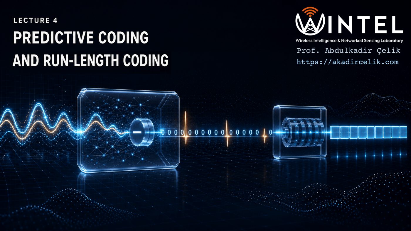
Lecture 3 showed that entropy-coding a memory source directly is wasteful. This lecture closes the loop: remove redundancy with a predictor, then compress the mostly-zero residual with run-length coding (RLC) — a lossless scheme with fixed-length output instead of the variable-length output of Shannon-Fano and Huffman.
- Apply predictive coding to remove redundancy from a correlated source before coding
- Design a run-length code for sources with long repeated runs and compute its efficiency
- Compare predictive and run-length strategies across different source statistics
Contents
This page grows as further lectures are added to the document.
4.1 Getting close to the information rate: removing redundancy
Predict first, then entropy-code
Any transmitted rate \(R_b\) demands bandwidth and power in proportion to its size, so source coding aims to push \(R_b\) as low as possible — ideally down to the source's true information rate. For a memoryless source, Lecture 2's entropy coding (Shannon-Fano, Huffman) already gets \(R_b\) close to that limit. Lecture 3 showed why the same trick fails for a source with memory: entropy-coding \(\{S(k)\}\) symbol by symbol only ever sees the one-symbol statistics, so it reaches \(R_s H(1)\), not the true (and much smaller) information rate \(R_s H\).
The fix is to attack the redundancy directly, before entropy coding: build a predictor for \(S(k)\) from its recent past \(\{S(k-i)\}_{i\ge1}\), subtract the prediction off, and code only what is left. Two application areas make this concrete:
- Speech coding: consecutive samples are highly correlated; a predictive model \(s(k)=\sum_{j=1}^q a_j s(k-j)+\varepsilon(k)\) (Lecture 3, Section 2.2) removes the predictable part, leaving an innovation \(\varepsilon(k)\) that is close to uncorrelated and zero-mean. The coder sends the small set of model parameters \(a_j\) together with \(\varepsilon(k)\), not \(s(k)\) itself.
- Video coding: a sequence of frames has both inter-frame (temporal, between frames) and intra-frame (spatial, within a frame) redundancy. Removing both leaves a much smaller residual to code.
Whatever the source, once the predictable part is removed, the resulting residual sequence is well suited to a further, purely lossless compression step. When that residual is binary and overwhelmingly zeros, as it typically is after a good predictor, run-length coding (RLC) is the natural tool.
4.2 A predictive scheme with run-length coding
The complete coding chain
Put together, redundancy removal and RLC form a complete coding chain for a memory source:
The predictor and its inverse must be identical at encoder and decoder (or the decoder must receive whatever side information the predictor needs), so that the residual \(e(i)\) reconstructs \(x(i)\) exactly on the decoding side, after RLC has been undone.
4.3 Run-length coding: building the codeword table
Runs of zeros, indexed into fixed codewords
RLC replaces a run of zeros followed by a one (or, for the very longest runs, a run with no terminating one at all) with a single, fixed-length codeword of \(n\) bits. Table entries are indexed by the run length \(l\), covering \(0 \le l \le N-1\) where \(N=2^n-1\):
| length of 0-run, \(l\) | encoder input pattern | encoder output codeword (\(n\) bits) |
|---|---|---|
| 0 | 1 | 00…000 |
| 1 | 01 | 00…001 |
| 2 | 001 | 00…010 |
| 3 | 0001 | 00…011 |
| ⋮ | ⋮ | ⋮ |
| \(N-2\) | 0…01 | 11…101 |
| \(N-1\) | 00…01 | 11…110 |
| \(N=2^n{-}1\) | 00…00 (no terminating 1) | 11…111 |
The whole scheme rests on one assumption: the input bit stream is mostly "0"s, i.e. \(p=P(\text{“0”})\) is close to 1. Then short runs (small \(l\)) dominate, so on average the encoder replaces a variable-length input pattern (often much longer than \(n\) bits) with a fixed, small \(n\)-bit codeword — that trade is where the compression comes from.
4.4 RLC efficiency
Average input length and compression ratio
Each output codeword is exactly \(n\) bits, so all that varies is how many input bits that codeword replaces. Averaging the input pattern length \(l+1\) over the geometric distribution of run lengths (probability \(p^l(1-p)\) of a run of exactly \(l\) zeros, plus probability \(p^N\) of the maximal all-zero run):
The compression ratio is then the average input length divided by the fixed output length:
4.4.1 RLC re-examined: variable in, fixed out
It is worth contrasting RLC's shape with Shannon-Fano and Huffman coding directly:
Despite this apparent reversal, both are governed by the same underlying principle: a rare event should map to a large codeword (relatively speaking), and a probable event to a small one. The cleanest way to see this is to define \(\text{ratio} = \dfrac{\text{output length}}{\text{input length}}\): a long run of zeros (high probability under the "mostly zero" assumption) maps to a small ratio, while a short run (lower probability) maps to a larger ratio. RLC, Shannon-Fano, and Huffman are all, in this sense, lossless (entropy) encodings.
4.5 Comparing RLC with Shannon-Fano and Huffman
Which side is held to a fixed length?
| Run-length coding | Shannon-Fano | Huffman | |
|---|---|---|---|
| Input length | variable (1 to \(N\) bits) | fixed (one symbol) | fixed (one symbol) |
| Output length | fixed (\(n\) bits) | variable, ≈ \(-\log_2 p_i\) | variable, ≈ \(-\log_2 p_i\) |
| Source it targets | binary, heavily skewed (\(p\to1\)) | general \(q\)-ary, any distribution | general \(q\)-ary, any distribution |
| Construction | fixed lookup table, indexed by run length | top-down recursive splitting | bottom-up greedy merging |
| Optimality | not optimal in general, but very cheap to run | usually close to optimal | provably optimal among prefix codes |
| Typical use | residual after prediction; fax; simple image formats | quick hand-built codes, teaching | general-purpose lossless compression (e.g. inside JPEG, ZIP) |
- All three are lossless: the original sequence can always be reconstructed exactly.
- Shannon-Fano and Huffman are suited to a general \(q\)-ary memoryless source with an arbitrary probability distribution; RLC is specialised to a binary source whose bits are heavily skewed toward "0" (or "1").
- RLC is the natural choice after a predictor has already removed the correlation from a memory source, since the resulting residual is typically binary and mostly zero — exactly the regime RLC is built for.
- Choosing \(n\) trades off compression ratio against worst-case pattern length: a larger \(n\) allows longer runs to be captured (raising \(N\) exponentially) but a single "1" still costs a full \(n\)-bit codeword, so \(n\) should be matched to how skewed \(p\) really is.
MATLAB corner
The script below generates a skewed binary residual, applies run-length coding by hand, and checks the empirical compression ratio against the closed-form formula.
Problems with solutions
Work each one before revealing the solution.
Summary and key formulas
- Removing redundancy first (a predictor) turns a memory source's residual into something close to memoryless, and, for binary residuals, heavily skewed toward zero.
- Run-length coding maps a run of up to \(N=2^n-1\) zeros (plus a terminating bit) onto a fixed \(n\)-bit codeword, trading a variable-length input for a fixed-length output.
- Compression ratio \(C=d/n=(1-p^N)/[n(1-p)]\) grows quickly as \(p\to1\); a well-chosen \(n\) balances this against the worst-case cost of a lone "1".
- RLC, Shannon-Fano, and Huffman are all lossless entropy-coding methods obeying the same rule — rare patterns cost more, relative to their length, than common ones — they simply differ in which side (input or output) is held fixed.
- Together, Lectures 1–4 now cover the complete source-coding toolkit for both memoryless and memory sources; Lecture 5 turns to what happens to information once it crosses a noisy channel.
Channels and Mutual Information
Lectures 1–4 asked how efficiently a source's information can be coded. This lecture asks what happens to that information once it crosses a noisy channel: how a channel is modelled, how input and output symbols relate through the binary symmetric channel, and how mutual information measures what actually gets through.
- Represent a noisy channel with a transition probability matrix
- Compute mutual information between channel input and output for a given source
- Explain how mutual information quantifies information conveyed through a noisy channel
Contents
This page grows as further lectures are added to the document.
5.1 Modelling the channel: AWGN and channel characteristics
An ideal path, corrupted only by noise
Every real channel can distort amplitude and phase, may vary with time, and has finite bandwidth \(B\). On top of that, error-free reception is impeded by additive white Gaussian noise (AWGN), whose severity is captured by the signal-to-noise ratio (SNR). Our aim in this lecture and the next is to find the maximum rate at which information can cross such a channel — the channel capacity — but first we need a working model of the channel itself.
5.1.1 The ideal channel and additive white Gaussian noise
An ideal channel introduces no amplitude or phase distortion — its impulse response is a pure delay, \(h(t)=\delta(t-T)\), giving flat magnitude response and linear phase (constant group delay). The only impairment left is AWGN: zero-mean, Gaussian-distributed noise with a flat ("white") power spectral density \(N_0/2\) over the channel bandwidth \(B\), giving total noise power \(N_P = N_0 B\). A non-ideal (dispersive) channel additionally distorts the signal, causing intersymbol interference; we set that complication aside and work with the ideal-channel-plus-AWGN model.
Physically, this noise arises largely at the receiver: the received signal is very weak by the time it arrives, so it must be amplified before its digital content can be detected, and that amplification itself introduces thermal noise (quantified by the amplifier's noise figure). Depending on the channel, we may treat it as memoryless (non-dispersive) or as having memory (dispersive) — we focus on the memoryless case.
5.1.2 Propagation in real channels: path loss, shadowing, and fading
The AWGN model captures the noise floor, but in a real wireless link the received signal power itself varies with distance and surroundings in three distinct, superimposed ways, each acting on a different physical scale:
5.1.3 From AWGN to the BSC: where the crossover probability comes from
The AWGN channel of Section 5.1.1 is continuous: send a voltage, receive that voltage plus a real-valued noise sample. The binary symmetric channel of Section 5.2 is discrete: send a bit, receive a bit that is occasionally flipped. These are not two rival models — the second is what the first becomes once you wrap a modulator and a detector around it. Understanding that step is what makes \(p_e\) a physical quantity rather than an arbitrary parameter.
With antipodal (BPSK) signalling the transmitter sends \(+\sqrt{E_b}\) for a "1" and \(-\sqrt{E_b}\) for a "0", where \(E_b\) is the energy per bit. The detector receives \(y = \pm\sqrt{E_b} + n\), with \(n\) a zero-mean Gaussian sample, and makes a hard decision: declare "1" if \(y>0\) and "0" otherwise. An error occurs precisely when the noise is large enough and of the right sign to carry \(y\) across the threshold, which happens with probability
So the chain AWGN + BPSK + hard decision is a binary symmetric channel, and \(p_e\) inherits its value from the physics of Section 5.1.1. This also shows what the BSC throws away: by keeping only the sign of \(y\), the detector discards how confident each decision was. Retaining that confidence — soft-decision decoding — is worth roughly 2 dB in practice, which is why the modern codes mentioned in Lecture 6 all use it. With that link established, we can study the discrete channel on its own terms.
5.2 The binary symmetric channel (BSC)
The discrete channel that AWGN becomes
Section 5.1.3 built the binary symmetric channel from the ground up: an AWGN path with a BPSK modulator and a hard-decision detector wrapped around it, carrying one of two input symbols \(X_0,X_1\) and producing one of two output symbols \(Y_0,Y_1\). "Symmetric" means the two ways of getting it wrong are equally likely, \(P(Y_1\mid X_0)=P(Y_0\mid X_1)=p_e\), the channel's error (crossover) probability.
Any joint event "\(X_i\) sent and \(Y_j\) received" has a joint probability linked to the conditionals by Bayes' rule:
5.3 Mutual information between a symbol pair
What does observing \(Y_j\) tell you about \(X_i\)?
Because \(Y_j\) and \(X_i\) are linked through the channel, they share information; that sharing is quantified by the mutual information of the pair:
Two extreme cases build the intuition.
(i) Perfect, noiseless channel (\(Y_i=X_i\)): every received symbol identifies its input with certainty, so \(P(X_i\mid Y_i)=1\) and
The channel conveys exactly the information content of \(X_i\); nothing is lost.
(ii) Extremely noisy channel (\(p_e=0.5\)): now \(Y_i\) is statistically independent of \(X_i\), so the joint probability factorises as \(P(X_i,Y_i)=P(X_i)\,P(Y_i)\) and the reverse conditional collapses onto the a priori probability:
Substituting into the definition, \(I(X_i,Y_i)=\log_2\frac{P(X_i)}{P(X_i)}=\log_2 1=0\) — the channel conveys nothing; all information is lost. In general \(0\le I(X_i,Y_i)\le I(X_i)\).
In general \(I(X_i)\ge I(X_i,Y_i)\): some information is lost whenever the channel is imperfect. Re-arranging the definition makes this explicit:
Here \(I(X_i\mid Y_j)\), the information content of \(X_i\) conditioned on having observed \(Y_j\), plays the role of an information-loss term. Rearranged once more, the three quantities line up as source information, information delivered, and information destroyed:
The bounds recover the two extreme cases above: zero loss for the perfect channel (\(I(X_i\mid Y_j)=0\)), and total loss \(I(X_i\mid Y_j)=I(X_i)\) when \(p_e=0.5\).
5.4 Average mutual information and information loss
What the receiver actually acquires
A single pair's mutual information is a per-symbol quantity; averaging over every possible input/output pair, weighted by the joint probability \(P(X_i,Y_j)\) with which that pair actually occurs, gives the average mutual information:
This is the average amount of source information the receiver actually acquires per received symbol, and must be distinguished from the source entropy \(H(X)\), the average information the source sends. By Bayes' rule the log-ratio can be written three equivalent ways — the identity that drives every simplification below:
5.4.1 Decomposing \(I(X,Y)\) into entropies
Split the logarithm of the ratio into two logarithms, then regroup each double sum. Using \(\sum_j P(X_i,Y_j)=P(X_i)\) on the first term and collecting the second term by output symbol (with \(P(X_i,Y_j)=P(Y_j)\,P(X_i\mid Y_j)\)):
The first sum is the source entropy \(H(X)\); the second is the equivocation \(H(X\mid Y)=\sum_j P(Y_j)\,H(X\mid Y_j)\), the average uncertainty about \(X\) that remains after \(Y\) is observed. An identical regrouping in terms of the output symbols yields the mirror-image form, so both decompositions hold:
The first form reads from the transmitter's side: what reaches the receiver equals what the source sends, \(H(X)\), minus the equivocation \(H(X\mid Y)\) lost in the channel. The second reads from the receiver's side: the same conveyed information equals the destination entropy \(H(Y)\) minus the error entropy \(H(Y\mid X)\) injected purely by channel noise. Both describe one physical quantity viewed from opposite ends of the channel.
MATLAB corner
The script below reproduces the worked example end to end: joint probabilities, per-pair mutual information, average mutual information, and the \(H(X)-H(X\mid Y)\) check.
Problems with solutions
Work each one before revealing the solution.
Summary and key formulas
- The BSC is what AWGN becomes once a BPSK modulator and a hard-decision detector are wrapped around it: the continuous received voltage collapses to one bit, and the noise density becomes a single symmetric crossover probability \(p_e=Q\big(\sqrt{2E_b/N_0}\big)\).
- Mutual information \(I(X_i,Y_j)\) measures how much observing \(Y_j\) tells you about \(X_i\): positive and near \(I(X_i)\) for likely (correct) pairs, negative ("mis-information") for error pairs.
- Average mutual information \(I(X,Y)\) is the true bits/symbol the receiver acquires, always \(\le H(X)\), with equality only for a noiseless channel.
- Two equivalent decompositions, \(I(X,Y)=H(X)-H(X\mid Y)=H(Y)-H(Y\mid X)\), tie mutual information to the entropies of source and destination.
- Next, in Lecture 6: maximising \(I(X,Y)\) over all possible source distributions defines the channel capacity — the fastest rate at which information can cross the channel error-free.
Channel Capacity
Lecture 5 defined mutual information, what a receiver actually learns per symbol. This lecture maximises it: the channel capacity \(C\) is the fastest rate at which information can cross a channel with arbitrarily small error, for both discrete channels (the BSC) and continuous ones (the Gaussian channel, via the Shannon-Hartley law).
- Derive channel capacity as the maximum mutual information over all input distributions
- Compute the capacity of the binary symmetric channel and other simple models
- Interpret the Shannon capacity theorem’s implications for error-free transmission rates
Contents
This page grows as further lectures are added to the document.
6.1 From mutual information to channel capacity
The best this channel could ever do
Lecture 5 defined average mutual information \(I(X,Y)\): the true bits/symbol a receiver acquires through a given channel, for a given source distribution. But different source distributions feeding the same channel give different values of \(I(X,Y)\). Shannon's channel capacity asks: over every possible input distribution, what is the most information this channel could ever convey?
If symbol \(X_i\) has duration \(t_i\) and \(t_{av}=\sum_i P(X_i)t_i\) is the average symbol duration, capacity in bits/second follows directly:
Two conditions jointly maximise \(I(X,Y)\): the channel must introduce no errors (\(H(Y\mid X)=0\)), and, whenever symbol durations are constant, the input symbols must be equiprobable. The first is a property of the channel, not something we control; the second is exactly the maximum-entropy condition from Lecture 3, now applied at the channel input.
6.1.1 Where "the channel" sits in the full system
It helps to place \(X(k)\) and \(Y(k)\) in the whole chain. The source emits symbols \(\{X_i\}\); the MODEM converts these to a continuous-time waveform \(x(t)\), which crosses the physical, continuous-time (analogue) channel and is demodulated back into a continuous waveform \(y(t)\), from which the receiver recovers symbols \(\{Y_i\}\).
6.2 Capacity of discrete channels
The noise-free bound, and the capacity of the BSC
6.2.1 The noise-free case
With no errors the error entropy vanishes, \(H(Y\mid X)=0\), so \(I(X,Y)=H(Y)=H(X)\): the channel conveys exactly the source entropy. Writing the source entropy and the average symbol duration explicitly,
so the capacity in bits/second is \(C=\max\{H(X)/t_{av}\}\). With constant symbol durations \(t_i=T_s\), the maximum entropy is reached by a memoryless, equiprobable \(q\)-ary source, for which \(H(X)=\log_2 q\), giving the maximum achievable transmission rate:
6.2.2 Capacity of the binary symmetric channel
For the BSC of Lecture 5 with equiprobable input, \(P(X_0)=P(X_1)=0.5\), symmetry forces \(P(Y_0)=P(Y_1)=0.5\) too. Working through the joint probabilities \(P(X_i,Y_j)\) and substituting into \(I(X,Y)\) (each of the four terms collapses to \(\log_2[2(1-p_e)]\) or \(\log_2(2p_e)\), matching Lecture 5's Problem 1 derivation) gives a capacity that depends on \(p_e\) alone:
Take equiprobable inputs \(P(X_0)=P(X_1)=\tfrac12\); by symmetry \(P(Y_0)=P(Y_1)=\tfrac12\). The four joint probabilities are
Write the average mutual information over the four \((i,j)\) pairs, using Bayes' rule \(\dfrac{P(X_i\mid Y_j)}{P(X_i)}=\dfrac{P(Y_j\mid X_i)}{P(Y_j)}\):
Substitute the values. With \(P(Y_j)=\tfrac12\), each ratio becomes \(2\,P(Y_j\mid X_i)\), so the four terms are
Collect the two identical correct-reception terms and the two identical error terms, then expand \(\log_2(2x)=1+\log_2 x\):
The two extremes match intuition directly: a perfect channel (\(p_e=0\)) gives \(C=1\) bit/symbol, the maximum possible for a binary alphabet; a maximally noisy channel (\(p_e=0.5\), output independent of input) gives \(C=0\) — no information can cross at all.
6.3 Shannon's channel coding theorem
Noise limits the rate, not the reliability
If the information rate \(R\) satisfies \(R \le C\), there exists a channel coding technique that transmits information over the channel with arbitrarily small error probability. If \(R > C\), error-free transmission is impossible.
This is one of the most consequential results in engineering: a noisy channel is not an obstacle to reliable communication, only a limit on the rate at which it can happen. Note carefully what the theorem does not say: it guarantees that a good code exists, but gives no recipe for constructing one. Most practical channel codes fall well short of \(C\), though capacity-approaching codes exist (e.g. turbo codes, low-density parity-check codes), and modern iterative turbo detection-decoding pushes real systems increasingly close to the Shannon limit.
6.4 Analogue sources and the Gaussian channel
Differential entropy, and why Gaussian maximises it
Real channels usually carry continuous-valued (analogue) signals, not discrete symbols, so we need an analogue counterpart to entropy. For a continuous source with probability density function \(p(x)\), the differential entropy is:
Just as a discrete source's entropy is maximised by an equiprobable distribution, Shannon showed that, among all continuous distributions with a given variance (power), differential entropy is maximised by the Gaussian PDF:
Because a Gaussian signal attains maximum entropy for its power, and because AWGN is itself Gaussian, it is natural to study the Gaussian channel: a channel input \(x\) with Gaussian PDF and power \(S_P=\sigma_x^2\), corrupted by independent AWGN \(\varepsilon\) with power \(N_P=\sigma_\varepsilon^2\).
A Gaussian signal passed through the linear operation "add independent Gaussian noise" remains Gaussian, so \(y=x+\varepsilon\) has power \(\sigma_y^2=S_P+N_P\) and its own maximum differential entropy \(H_{\max}(y)=\tfrac12\log_2\!\big(2\pi e(S_P+N_P)\big)\). Since \(I(x,y)=H(y)-H(y\mid x)\) and the residual uncertainty \(H(y\mid x)\) is exactly the noise's own entropy, \(H(y\mid x)=H(\varepsilon)=\tfrac12\log_2(2\pi e\,N_P)\), the two logarithm terms subtract cleanly:
and cancelling the common factor leaves the striking per-symbol capacity of the Gaussian channel:
6.5 The Shannon-Hartley law and the bandwidth/SNR trade-off
Bandwidth and power, traded against each other
Sampling the Gaussian channel at the Nyquist rate \(f_s=2B\) converts the per-symbol result of Section 4 into a rate, giving the celebrated Shannon-Hartley law:
where \(B\) is the channel bandwidth in Hz and \(N_P=N_0 B\) with \(N_0\) the (two-sided) AWGN power spectral density. This is often an excellent approximation for practical digital channels, even ones that are not exactly Gaussian.
Two, and only two, physical resources set the capacity: bandwidth \(B\) and signal power \(S_P\) (via the SNR). Either can be traded for the other while holding \(C\) fixed — a noiseless channel (\(S_P/N_P\to\infty\)) has infinite capacity, but capacity does not diverge as \(B\to\infty\) with fixed \(S_P,N_0\); it approaches a finite ceiling:
MATLAB corner
The script below plots BSC capacity against \(p_e\) and evaluates the Shannon-Hartley law for the worked example.
Problems with solutions
Work each one before revealing the solution.
Summary and key formulas
- Channel capacity is the maximum of \(I(X,Y)\) over all input distributions — a property of the channel alone, achieved only by the right (typically equiprobable) source.
- The BSC's capacity falls from 1 bit/symbol at \(p_e=0\) to 0 at \(p_e=0.5\), dropping steeply even for small error rates.
- Shannon's theorem guarantees arbitrarily reliable transmission below capacity, but does not construct the code; practical capacity-approaching codes (turbo, LDPC) exist but are hard to design.
- Gaussian signals maximise differential entropy for a given power, making the Gaussian channel the natural continuous-channel model, with \(I(x,y)=\tfrac12\log_2(1+S_P/N_P)\).
- The Shannon-Hartley law converts this into bits/second, and shows bandwidth and SNR can be traded for one another, though capacity grows only logarithmically in power versus linearly in bandwidth.
Wrap-up and Tutorial
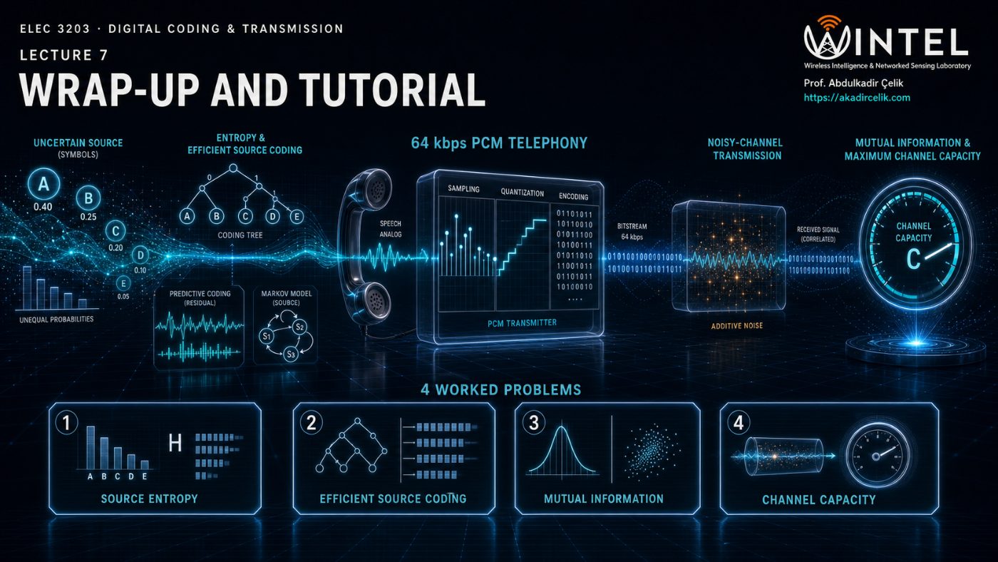
A single revision chapter that ties the whole module together: the source side (entropy, rates, efficient coding), the channel side (mutual information and capacity), a real-world case study — the 1960s 64 kbps telephone speech codec — and four fully worked, exam-style tutorial problems spanning every topic.
- Consolidate the module’s source-side and channel-side results into one end-to-end framework
- Apply entropy, efficiency, mutual-information and capacity formulas to worked tutorial problems
- Relate the theoretical results to a practical system case study
Contents
Revision of the whole module, a practical case study, then four detailed tutorial problems.
7.1 Revision — the source side
Everything the source side asks of you
A digital source is fully specified by four things: its symbol set, the probability of each symbol, its symbol rate, and any interdependency between successive symbols. Source coding turns that stream of symbols into a stream of bits — ideally as few bits as the information content allows.
| Quantity | Formula | Meaning |
|---|---|---|
| Information content | \(I(m_i)=-\log_2 p_i\) | bits carried by one occurrence of symbol \(m_i\) |
| Entropy (memoryless) | \(H=-\sum_{i=1}^{q} p_i\log_2 p_i\) | average information per symbol |
| Entropy (1st-order Markov) | \(H=\sum_i p_i H_i=-\sum_i p_i\sum_j p_{ij}\log_2 p_{ij}\) | state-averaged entropy with memory |
| Information rate | \(R=R_s\,H\) | bits/s the source really needs to send |
| Coding efficiency | \(\eta = R / R_b = H/\bar L\) | how close the coded rate gets to \(R\) |
Efficient source coding aims to get the coded bit rate \(R_b\) as close as possible to the information rate \(R\). For a memoryless source, apply entropy coding (Shannon-Fano, Huffman), or run-length coding if the source is binary with mostly zeros. For a source with memory, you must first remove the redundancy — that is the subject of the next section.
7.2 Practical source coding: remove redundancy first
Always the same two steps
Entropy coding is optimal only for a memoryless source. Real signals — speech, images, video — are highly correlated, so the winning strategy is always the same two steps:
Remove the predictable part with a model (e.g. a predictor). The residual left over is nearly white — almost memoryless.
Apply Shannon-Fano or Huffman to the residual — or RLC if it is binary with mostly zeros. Now entropy coding is near-optimal.
Speech has strong temporal correlation; video adds spatial (intra-frame) correlation on top of temporal (inter-frame) correlation. A video coder, for instance, sends one whole reference frame and then only the frame-to-frame difference — itself often run-length coded. Whenever you meet a practical codec, look for these two steps.
7.3 Revision — the channel side
One channel, seen two ways
Depending on which part of the system you look at, the channel is either discrete-time (symbols in, symbols out, across the modem) or continuous-time (the analogue waveform channel inside it).
Average mutual information \(I(X,Y)\) characterises what happens to information as it crosses the channel, and splits two equivalent ways — from the transmitter's side and from the receiver's side:
7.4 Channel capacity at a glance
Four channels, four formulas
Channel capacity \(C\) is the maximum error-free information rate a channel can carry. Shannon's theorem: if the source information rate \(R\le C\), a coding scheme exists that transmits with arbitrarily small error; if \(R>C\), error-free transmission is impossible.
| Channel | Capacity | Notes |
|---|---|---|
| Discrete, general | \(C=\max\{I(X,Y)\}\) | max over input distributions; also \(C/T_{av}\) in bits/s |
| Noise-free \(q\)-ary | \(C=\log_2 q / T_s\) | equiprobable symbols, constant duration \(T_s\) |
| BSC | \(C=1+(1-p_e)\log_2(1-p_e)+p_e\log_2 p_e\) | \(C{=}1\) at \(p_e{=}0\); \(C{=}0\) at \(p_e{=}0.5\) |
| Gaussian (Shannon-Hartley) | \(C=B\log_2\!\left(1+\dfrac{S_P}{N_P}\right)\) | \(N_P=N_0 B\); trade bandwidth \(B\) against power \(S_P\) |
7.5 Case study
The 1960s 64 kbps telephone speech codec
When the analogue telephone network was digitised, speech was coded at a fixed 64 kbps. The pipeline: band-limit to 3.4 kHz, sample at 8 kHz, pass through a μ-law compressor, then quantise to 8 bits (256 levels).
Tutorial: worked Examples 1–4
Four exam-style problems spanning the whole module. Each is stated exactly as in the course, then solved in full — work through it before revealing the solution.