ELEC3203 · Digital Coding and Transmission

Lecture 1

Information,
Entropy and the Digital Source

How much information does a message actually carry, and what is the smallest number of bits we truly need in order to send it? This lecture builds the answer from first principles.

Learning Objectives

• Explain the anatomy of a digital communication system (Tx, channel, Rx) and where information theory fits
• Compute the self-information and entropy of a discrete memoryless source
• Calculate a source’s information rate and explain why fixed-length BCD coding wastes bandwidth

SlidesQuiz

Podcast

InstructorProf. Abdulkadir Çelik https://akadircelik.com ModuleELEC3203 TopicsInformation · entropy · information rate · source coding

▸ Information content ▸ Entropy ▸ Memoryless sources ▸ Information rate

1.1  A primer on digital communication systems

The whole module in miniature — transmitter, channel, receiver, and the resources they trade

The aim of any telecommunication system is to convey information between two locations that are separated in space, over a channel of adequate quality, at a certain rate and reliably.

This picture is the whole module in miniature. The channel offers a fixed set of resources — transmit power, time, and bandwidth (and, in multi-antenna systems, space) — and the job of the transmitter and receiver design is to spend those resources so as to hit the best possible key performance indicators (KPIs): information rate (how many bits per second get through), latency (how long it takes), reliability (how rarely errors slip past), and energy efficiency (how many bits per joule). Every technique in this module, from source coding to channel coding to modulation, is really a way of trading these resources for these KPIs.

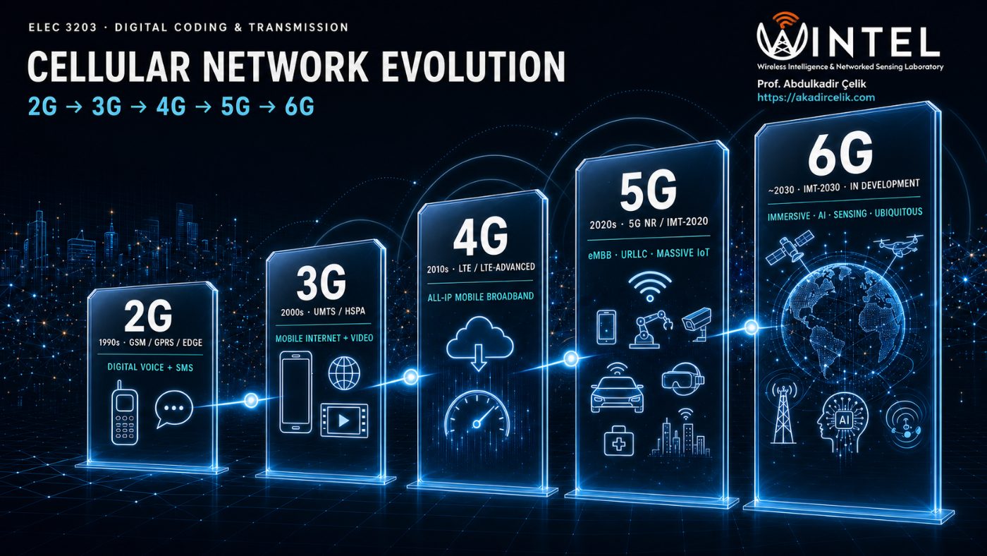
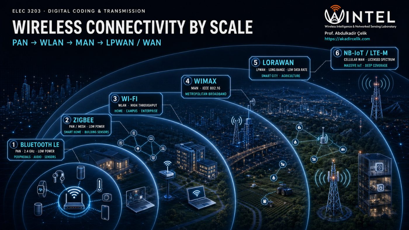
In practice there is no single "best" wireless technology — different applications sit at different points on the resource/KPI trade-off, so the wireless landscape has evolved into a family of standards, each tuned to a different range, data rate, power budget, and device density. Cellular networks (2G–6G) have progressively traded new spectrum and complexity for higher rate, lower latency, and support for ever more connected devices, while short- and medium-range technologies (Bluetooth LE, Zigbee, Wi-Fi, WiMAX, LoRaWAN, NB-IoT) each cover a different rung of the range/power/throughput ladder, from a wrist-worn sensor a few metres away to a smart-city meter kilometres from its gateway.

Because the whole module is digital, we first look at how a real source becomes a stream of bits, and then place that stream in the full system.

An analogue source such as speech or video is not digital to begin with. It is turned into a stream of bits by two steps:

With the source reduced to a clean stream of bits, we can place it in the full communication system. A generic digital transmission scheme is a chain of building blocks, with the transmitter along the top, the channel on the right, and the receiver returning along the bottom.

This lecture concentrates on the very first block, the source, and asks the most basic question of the whole field. What is information, and how do we measure it?

1.2  What is information?

Surprise as a measurable quantity

Consider a weather forecast of rain tomorrow in three places:

The same three words, "it will rain", carry wildly different amounts of information. The rainforest forecast tells us almost nothing, because we knew it already. The desert forecast is a genuine shock. This is the central intuition: information is tied to uncertainty. The more unexpected an event is, meaning the smaller its probability, the more information its occurrence conveys. That single idea is the seed of the entire theory.

1.3  Information content of a symbol

Three requirements pin down the function

We want a function \(I(m_i)\) of a symbol's probability \(p_i\) that behaves the way our intuition demands. Three requirements pin it down:

• Monotone in surprise: A smaller \(p_i\) should give a larger \(I\).
• Certainty carries nothing: We need \(I = 0\) when \(p_i = 1\).
• Additive for independent events: Two independent symbols occurring together, with probability \(p_i p_j\), should carry information \(I(m_i) + I(m_j)\). (A short proof that only the logarithm can satisfy this is given in the appendix.)

The additivity requirement is the decisive one. We need \(I(p_i p_j) = I(p_i) + I(p_j)\), that is, a function that turns products into sums. That is exactly the defining property of the logarithm, so \(I(p) \propto \log(1/p)\). Choosing base 2 fixes the unit as the bit:

The properties follow immediately from the graph of \(-\log_2 p\):

• Since \(0 \le p_i \le 1\), we have \(I(m_i) \ge 0\), so information is never negative.
• If \(p_i > p_j\), then \(I(m_i) < I(m_j)\), so rarer symbols carry more.
• \(I(m_i) \to 0\) as \(p_i \to 1\), so a certain symbol carries no information.
• \(I(m_i) \to \infty\) as \(p_i \to 0\), so a vanishingly rare symbol carries unbounded information, although it almost never occurs.

1.3.1  Physical interpretation: bits as binary digits

Why "bits"? Because the information content of a symbol equals the smallest number of binary digits needed to label it, in the case where symbols are equally likely:

• 2 equally likely symbols \(\{0,1\}\): one binary digit each, and \(I = \log_2 2 = 1\) bit. ✓
• 4 equally likely symbols \(\{00,01,10,11\}\): two digits each, and \(I = \log_2 4 = 2\) bits. ✓
• \(q\) equally likely symbols: \(\log_2 q\) digits each, and \(I = \log_2 q\) bits. ✓

Assigning \(\log_2 q\) bits to every symbol is called Binary Coded Decimal (BCD). It is exactly right when symbols are equally likely. When they are not, it wastes bits, and fixing that waste is what the rest of Lectures 1 to 4 are about.

1.4  Entropy

Average information per symbol

A single symbol's information varies from one symbol to the next. What matters for system design is the average. Take a long sequence of \(N\) symbols from a memoryless source. Because the symbols are independent and \(N\) is large, symbol \(m_i\) appears about \(p_i N\) times.

Information from symbol \(m_i\) across the whole sequence. It occurs \(p_i N\) times, each occurrence worth \(I(m_i)\):

Total information in the sequence, summed over the alphabet:

Average information per symbol. Divide by \(N\), and \(N\) cancels. This average is the entropy \(H\):

Entropy is a fundamental physical property of the source. It depends only on the alphabet and the probabilities, that is on quantities 1, 2 and 4, and not on the symbol rate. It answers a clear question: on average, how many bits of genuine information does each symbol carry?

1.4.1  The binary source and maximum entropy

For a binary source with \(P(1)=p\) and \(P(0)=1-p\), the entropy is the binary entropy function:

Its shape is worth memorising. It is zero at both ends, because a biased coin that almost always lands the same way is predictable and so carries almost no information. It reaches a single maximum of exactly 1 bit at \(p = 0.5\), the fair coin, which is the point of greatest uncertainty.

This generalises. For a \(q\)-ary source, entropy is greatest when all symbols are equally likely, so \(p_i = 1/q\) and \(H_{\max} = \log_2 q\). This gives the key bound, which we revisit throughout the module:

1.5  Information rate

From bits per symbol to bits per second

Entropy is measured per symbol. Multiply it by the symbol rate \(R_s\) to find how many bits of real information the source produces per second. This is the information rate:

Unlike entropy, the information rate depends on all four source quantities, because it includes \(R_s\). It is the true, irreducible demand of the source in bits per second, and it is the target that any good encoder tries to hit.

1.6  Why BCD wastes bandwidth

Sending more bits than you need

If we simply encode every symbol with \(\log_2 q\) bits, which is BCD, the source's output bit rate is:

Since \(H \le \log_2 q\), it follows at once that

So the number of bits we actually send, \(R_b\), is generally larger than the number we truly need to send, \(R\). The gap \(R_b - R\) is pure waste. It matters because, as later lectures show, transmitting at \(R_b\) bits per second costs real resources, namely bandwidth and power. Squeezing \(R_b\) down toward \(R\) is the whole business of efficient source coding, the subject of Lecture 2, which covers Shannon and Fano coding and Huffman coding.

Worked examples

MATLAB corner

Three short scripts make the ideas concrete: a reusable entropy function, a plot of the binary entropy curve so you can see the peak at \(p = 0.5\) for yourself, and a real-data check using English letter frequencies.

% Entropy (bits/symbol) of a discrete memoryless source.
% p : vector of symbol probabilities (must sum to 1).
function H = entropy_bits(p)
    p = p(p > 0);            % drop zeros: 0*log2(0) := 0
    if abs(sum(p) - 1) > 1e-9
        warning('Probabilities do not sum to 1.');
    end
    H = -sum(p .* log2(p));
end
 
% --- Example 1.2 check ---
p = [1/2 1/4 1/8 1/8];
H = entropy_bits(p)          % H = 1.7500
Rs = 1000;  R = Rs * H       % R = 1750 bits/s
Rb = Rs * log2(numel(p))     % Rb = 2000 bits/s
eff = H / log2(numel(p))     % eff = 0.8750

% Binary entropy function H(p) = -p*log2(p) - (1-p)*log2(1-p)
p = linspace(0, 1, 501);
H = -p.*log2(p) - (1-p).*log2(1-p);
H(isnan(H)) = 0;             % fix the endpoints p = 0, 1
 
plot(p, H, 'LineWidth', 2); grid on
xlabel('P(1) = p'); ylabel('H(p)  [bits/symbol]');
title('Binary entropy function');
[Hmax, k] = max(H);
fprintf('Peak H = %.3f bit at p = %.2f\n', Hmax, p(k));
% Peak H = 1.000 bit at p = 0.50

% Entropy of English text from single-letter frequencies
% (a classic unigram table, percent occurrence, order ETAOIN...).
letters = 'ETAOINSHRDLCUMWFGYPBVKJXQZ';
freq = [12.70 9.06 8.17 7.51 6.97 6.75 6.33 6.09 5.99 4.25 ...
        4.03 2.78 2.76 2.41 2.36 2.23 2.02 1.97 1.93 1.29 ...
        0.98 0.77 0.15 0.15 0.10 0.07];
p = freq / sum(freq);
 
H    = entropy_bits(p)        % H    = 4.1717 bits/letter
Hmax = log2(numel(p))         % Hmax = 4.7004 bits/letter (BCD, equiprobable)
 
fprintf('English (unigram): %.2f bits/letter vs BCD %.2f bits/letter\n', H, Hmax);
% English (unigram): 4.17 bits/letter vs BCD 4.70 bits/letter

Problems with solutions

Work each one before reading the solution.

Summary and key formulas

• Information measures surprise. Rarer symbols carry more, and the unit is the bit.
• Entropy is the average information per symbol, a fundamental property of the source that does not depend on the symbol rate.
• Information rate \(R = R_sH\) is the true number of bits per second the source must send.
• BCD spends \(\log_2 q\) bits per symbol and is optimal only for equally likely sources. In general \(R_b \ge R\), which leaves room for efficient coding.
• Next, in Lecture 2: maximum entropy, and building efficient codes with the Shannon and Fano method and Huffman coding, which push \(\bar L\) down toward \(H\).

Appendix: why the logarithm?

Section 3 asked for a function \(I(p)\) with three properties: it decreases as \(p\) increases, it vanishes at \(p=1\), and it is additive, \(I(p_ip_j) = I(p_i) + I(p_j)\), for independent events. Here we show the additivity condition alone, together with the mildest smoothness assumption, forces \(I\) to be a constant multiple of \(\log(1/p)\).

Step 1. Restate additivity as a functional equation. Write \(f(p) = I(p)\) for \(p \in (0,1]\). The requirement is

Step 2. Substitute \(x = y\). Then \(f(x^2) = 2f(x)\), and by induction \(f(x^n) = nf(x)\) for every positive integer \(n\). Applying this with \(x\) replaced by \(x^{1/n}\) gives \(f(x) = n f(x^{1/n})\), so also \(f(x^{m/n}) = \tfrac{m}{n} f(x)\) for positive integers \(m, n\). So \(f(x^r) = r f(x)\) for every positive rational \(r\), and by continuity (our smoothness assumption) for every real \(r > 0\).

Step 3. Fix a reference point. Pick any \(x_0 \in (0,1)\) and define the constant \(c = f(x_0)/\ln(1/x_0) > 0\) (positive because \(f\) decreases and \(\ln(1/x_0) > 0\)). For any other \(p \in (0,1)\) write \(p = x_0^r\) for \(r = \ln p / \ln x_0\). Then by Step 2:

Step 4. Conclude. So \(f(p) = c\ln(1/p)\) for some positive constant \(c\), that is, \(I(p)\) must be a constant multiple of a logarithm of \(1/p\), in any base. Choosing \(c = 1/\ln 2\) turns the constant into \(\log_2\) and fixes the unit as the bit:

No other family of functions, polynomial, exponential, or otherwise, satisfies the additivity requirement. The logarithm is not a convenient modelling choice; it is the only function the axioms allow.