ELEC6218 · Signal ProcessingAnalog & Digital Filter Design
Signal Processing · Lecture notesProf. Çelik
ELEC6218 · Signal Processing
Lecture 7
FIR Filter Design
This lecture shows how to design a practical FIR filter with linear phase. We first use symmetry to understand the four FIR types. We then compare two design routes: the window method, which is simple and flexible, and the minimax method, which makes the best use of a chosen filter order.
InstructorProf. Abdulkadir Çelik (https://akadircelik.com)ModuleELEC6218TopicsLinear-phase Types I–IV · minimax & Parks–McClellan · window method · Kaiser window · order estimation
▸ Symmetry, not luck, buys linear phase▸ Type II/III/IV each forbid one shape▸ Windowing: truncate, then taper▸ Minimax spreads the error evenly
Learning outcomes
By the end of this lecture, you will be able to:
Identify FIR Types I–IV from the order and coefficient symmetry, and decide which filter responses each type can realize.
Explain what minimax and equiripple mean, and describe how the Parks–McClellan algorithm reduces the largest weighted error.
Use the window method to turn an ideal sinc response into a finite causal filter, and choose a fixed or Kaiser window for a given attenuation.
Convert frequency and ripple specifications into an estimated filter order, construct the coefficients, and verify the result.
Lecture 7
Contents
First, learn how coefficient symmetry creates four linear-phase FIR types. Then compare the equiripple and window methods through complete numerical examples. The final section turns the window method into a reusable design checklist.
iNotation used in this lecture
\(M\)
filter order (Lecture 6 notation); length \(L=M+1\)
\(A(e^{j\omega})\)
real-valued amplitude function left after the linear-phase factor \(e^{-j\omega M/2}\) is pulled out
\(\delta_p,\delta_s\)
passband and stopband ripple (linear); \(A_p,A_s\) their dB equivalents
\(\omega_p,\omega_s\)
passband edge and stopband edge (rad/sample); \(\Delta\omega=\omega_s-\omega_p\)
\(w[n]\)
window function multiplying the ideal (infinite) impulse response
\(\beta\)
Kaiser window shape parameter
Most designs here use Type I or Type II. Their even symmetry suits ordinary low-pass, high-pass, band-pass and band-stop filters. Odd-symmetry Types III and IV are mainly used for differentiators and Hilbert transformers.
7.1 Linear-phase FIR filters: the four types
An FIR filter has generalized linear phase when its coefficients are symmetric or antisymmetric. Combining the two symmetry choices with even or odd order gives four FIR types. Each type has a constant group delay, but some types force the response to be zero at DC or at the Nyquist frequency.
$$ H(e^{j\omega})=A(e^{j\omega})\,e^{-j\alpha\omega+j\beta}, \qquad \alpha=\text{constant group delay} $$
(7.1)
In every case, the group delay is \(\alpha=M/2\). Even symmetry produces cosine terms and \(\beta=0\); odd symmetry produces sine terms and \(\beta=\pi/2\). The sign of the real amplitude function \(A(e^{j\omega})\) may change across a zero.
7.1.1 Type I: \(M\) even, even symmetry — the general-purpose case
\(h[n]=h[M-n]\), symmetric about the integer sample \(n=M/2\). Pairing terms \(k\) and \(M-k\) in the frequency-response sum and factoring out \(e^{-j\omega M/2}\) collapses every pair into a single cosine:
Type I does not force a zero at either \(\omega=0\) or \(\omega=\pi\). It can therefore realize low-pass, high-pass, band-pass and band-stop responses, making it the most flexible type.
7.1.2 Type II: \(M\) odd, even symmetry — no high-pass
Same symmetry, but with \(M\) odd the centre of symmetry \(M/2\) falls halfway between two samples, so the pairing gives half-integer cosine arguments instead:
At \(\omega=\pi\), every cosine term is zero, so Type II always has \(H(e^{j\pi})=0\). The forced zero at \(z=-1\) prevents a high-pass response, because a high-pass filter must pass frequencies near Nyquist. Type II is still suitable for low-pass and many band filters.
7.1.3 Type III: \(M\) even, odd symmetry — no low-pass or high-pass
\(h[n]=-h[M-n]\) (antisymmetric); the algebra now collapses into sines, with an overall factor of \(j\):
The sine terms vanish at both \(\omega=0\) and \(\omega=\pi\). Type III therefore has forced zeros at \(z=1\) and \(z=-1\), so it cannot realize an ordinary low-pass or high-pass response. It is commonly used for differentiators and Hilbert transformers.
7.1.4 Type IV: \(M\) odd, odd symmetry — no low-pass
Antisymmetric with \(M\) odd combines both effects: half-integer sine arguments, and only the DC zero survives (the half-integer argument never lands exactly on \(\pi k\)):
Type IV always has a zero at DC but does not force a zero at Nyquist. It cannot be a low-pass filter, but it is well suited to a digital differentiator, whose desired response is already zero at DC and increases with frequency.
The four types can be remembered visually: check whether the coefficients mirror or change sign, then check whether the symmetry centre lies on a sample or halfway between samples. Those two observations determine the type and its forced zeros.
Figure 7.1.a. Schematic impulse responses for the four linear-phase types: Types I/II mirror about the centre (even symmetry), Types III/IV flip sign about it (odd symmetry). The dashed line marks the symmetry centre — for even \(M\) it falls on a sample (an odd number of taps), for odd \(M\) it falls between two samples (an even number of taps), and Type III's centre sample is forced to zero (hollow marker). The forced zeros of Eqs. (7.3)–(7.5) are a direct consequence of this shape, not a separate design choice.
Type I
M even · even symmetry
No restriction. LPF, HPF, BPF, BSF all possible.
Type II
M odd · even symmetry
Forced zero at \(z=-1\). No HPF.
Type III
M even · odd symmetry
Forced zeros at \(z=\pm1\). No LPF or HPF.
Type IV
M odd · odd symmetry
Forced zero at \(z=1\). No LPF.
Figure 7.1.b. The four types and their consequences in the \(z\)-plane. Red crosses mark the zeros the symmetry forces onto the unit circle: one at \(z=1\) kills the DC gain, so no low-pass; one at \(z=-1\) kills the Nyquist response, so no high-pass. Type I forces neither and can realise any of the four shapes. Each filter also carries its designed zeros elsewhere in the plane, not drawn here.
None of this is bookkeeping. Given a set of taps you can now read off, in a few seconds and without evaluating a single frequency, whether the filter can possibly do the job it was handed — and if a specification asks for a high-pass from an even-length symmetric filter, you know to stop and change the length rather than to keep tuning coefficients. Example 7.1 walks that reading once, end to end.
EXAMPLE 7.1 · Classifying a filter and predicting its forbidden zero
A 5-tap filter has \(h=[1,\,2,\,0,\,-2,\,-1]\) (\(n=0,\ldots,4\)). Classify its type, predict any forced zero on the unit circle, and confirm it by evaluating \(H(e^{j\omega})\) at that frequency.
Step 1 · Order and symmetry. \(M=4\) (even). Check \(h[n]=-h[4-n]\): \(h[0]=1=-h[4]=-(-1)=1\ \checkmark\), \(h[1]=2=-h[3]=-(-2)=2\ \checkmark\), \(h[2]=0=-h[2]\ \checkmark\) (forces the centre tap to zero, as odd symmetry with even \(M\) always must). Odd symmetry, \(M\) even — Type III.
Step 2 · Predicted zeros. By Eq. (7.4), Type III forces \(H(e^{j0})=0\) and \(H(e^{j\pi})=0\) — zeros at both \(z=1\) and \(z=-1\), regardless of the coefficient values.
Step 3 · Confirm directly. \(H(z)=1+2z^{-1}+0-2z^{-3}-z^{-4}\). At \(z=1\): \(H(1)=1+2+0-2-1=0\ \checkmark\). At \(z=-1\): \(H(-1)=1-2+0+2-1=0\ \checkmark\). Both forced zeros confirmed — this filter can be neither a low-pass nor a high-pass, exactly as Section 7.1.3 predicts.
MATLAB corner for Example 7.1
This script checks Example 7.1's classification numerically: it verifies the antisymmetry, then uses roots() to show \(z=\pm1\) are exact roots of \(H(z)\).
Goal: confirm both forced zeros land exactly on the unit circle at \(z=1\) and \(z=-1\), for this filter and for a second, arbitrary Type III filter.
fir_type_zeros_demo.m
MATLAB
%% fir_type_zeros_demo.m - Example 7.1's Type III forced zeros (Eq. 7.4)
h = [120 -2 -1]; % M=4, odd (antisymmetric) about n=2
M = numel(h)-1;
% Step 1: verify antisymmetry h[n] = -h[M-n]
isAnti = isequal(h, -fliplr(h));
if mod(M,2)==0, ftype = 'III'; else, ftype = 'IV'; end
figure('Color','w'); zplane(h,1); title('Type III: zeros forced at z=\pm1');
Figure 7.1.c.Checking the Type III FIR zeros. MATLAB places one zero at \(z=1\) and another at \(z=-1\), both exactly on the unit circle. Evaluating the frequency response at these points gives \(H(e^{j0})=0\) and \(H(e^{j\pi})=0\). A Type III filter therefore has zero gain at DC and at the Nyquist frequency. These zeros are forced by odd symmetry; they are not approximate results of the numerical design.
So symmetry settles what a linear-phase FIR filter is allowed to do. It says nothing about how to choose the \(M+1\) coefficients that make it do the job well — and that is a great deal of freedom to spend by hand.
Two schools of thought answer this, and they differ in the one decision that matters: what error do you agree to make small? Everything else — the algebra, the algorithm, the order you end up paying for — follows from that single choice.
Section 7.2
Minimax — Parks–McClellan
Sections 7.3–7.4
Windowing — truncate and taper
Minimises
the worst-case weighted error, \(\max_\omega|W(\omega)E(\omega)|\) — the \(L_\infty\) norm.
the mean-squared error over frequency — the \(L_2\) norm.
Answer looks like
equal ripple everywhere: no band edge treated better than any other.
ripple largest at the band edge, dying away from it.
You get it by
solving a linear system and iterating (the Remez exchange) — running an algorithm.
writing down \(h_d[n]\,w[n]\): one formula, no iteration, no solver.
Pays with
no closed form, and an optimiser in the loop.
a handful of extra taps over the minimax optimum.
Buys
the provably lowest order meeting a given \(A_p,A_s,\Delta\omega\).
a design you can do on paper, predict, and re-tune with one parameter.
Neither dominates: they are optimal against different questions, and the \(L_\infty\)/\(L_2\) split is exactly why. Minimax spends its whole error budget uniformly, so nothing is wasted and nothing is spare; windowing lets the error pile up where the ideal response is discontinuous and be negligible elsewhere, which is a worse peak but a much simpler recipe. We take them in order of ambition — first the provably best filter of a given order, then the one you can write down — and Problem 7.3 asks you to argue which you would actually ship.
7.2 Minimax design: the Parks–McClellan algorithm
For a Type I filter, the design variables are the coefficients \(a[k]\) in the cosine sum \(A(\omega)\). The minimax criterion chooses them to make the largest weighted error over the specified passband and stopband as small as possible:
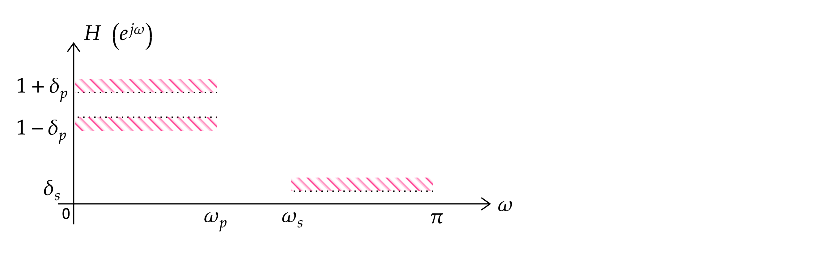
The set \(F\) contains the passband and stopband; the transition band is not constrained. The weighting function \(W(\omega)\) controls the relative importance of each band. Increasing a band's weight reduces its ripple, usually at the expense of larger ripple elsewhere.
Figure 7.2.a. The tolerance scheme Eq. (7.6) is written against: the design must stay inside the hatched corridors — \(1\pm\delta_p\) across the passband and \(\pm\delta_s\) across the stopband — while the transition band \(\omega_p<\omega<\omega_s\) is left completely unconstrained.
7.2.1 The Alternation Theorem
The Alternation Theorem identifies the optimum through the shape of its weighted error curve:
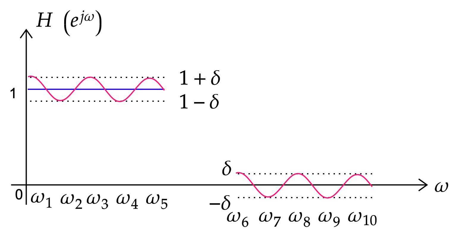
At the optimum, the weighted error reaches equal positive and negative peaks at a sufficient number of extremal frequencies. This is the equiripple pattern. It uses the available error allowance efficiently, so for a fixed order it gives the smallest possible worst-case error.
Figure 7.2.b. The Alternation Theorem's signature (Eq. 7.7), read off the response itself: at the optimum the deviation from the ideal touches its bound alternately — \(1+\delta\) then \(1-\delta\) across the passband, \(+\delta\) then \(-\delta\) across the stopband — at the \(N=M/2+2\) extremal frequencies \(\omega_1,\ldots,\omega_{10}\), and nowhere exceeds \(\delta\) in between. Equal-height ripples everywhere are what optimality looks like.
7.2.2 The Remez exchange algorithm
The Parks–McClellan method uses the Remez exchange algorithm to find this equiripple solution. MATLAB implements it in firpm():
1
Guess
Pick an initial set of \(N\) extremal frequencies \(\omega_1,\ldots,\omega_N\) — any reasonable spread across the bands will do.
2
Solve
With those frequencies held fixed, solve the linear system \(W(\omega_k)\big[H_d(\omega_k)-A(\omega_k)\big]=(-1)^k\delta\) for the coefficients \(a[k]\) and the ripple \(\delta\).
3
Locate the real extrema
With those coefficients fixed, search the resulting error curve for its true extremal frequencies \(\omega_k'\).
4
Exchange & repeat
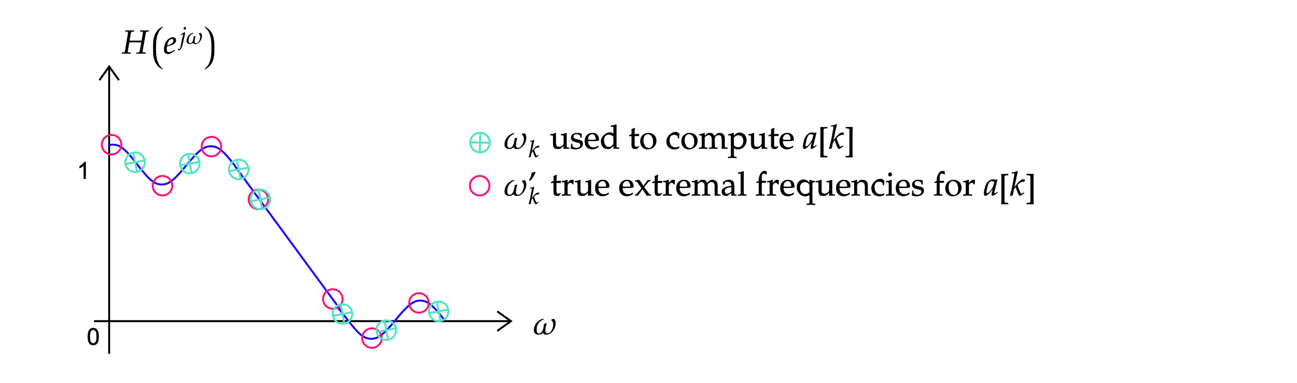
If \(\omega_k'\ne\omega_k\), replace \(\omega_k\) with \(\omega_k'\) and go back to step 2. This swap is the “exchange” in the algorithm’s name.
5
Converged
The frequencies stop moving: every ripple now has the same height, so by Eq. (7.7) the design is optimal.
Each iteration exchanges the guessed extremal set for a better one — hence “exchange” — and convergence is fast and guaranteed for this class of problem.
Figure 7.2.c. One step of the exchange. The \(\omega_k\) used to solve for \(a[k]\) (crossed markers) do not coincide with the true extremal frequencies \(\omega_k'\) of the error that results (open markers); replacing the former with the latter and re-solving is the whole algorithm, and the iteration stops when the two sets coincide.
MATLAB corner
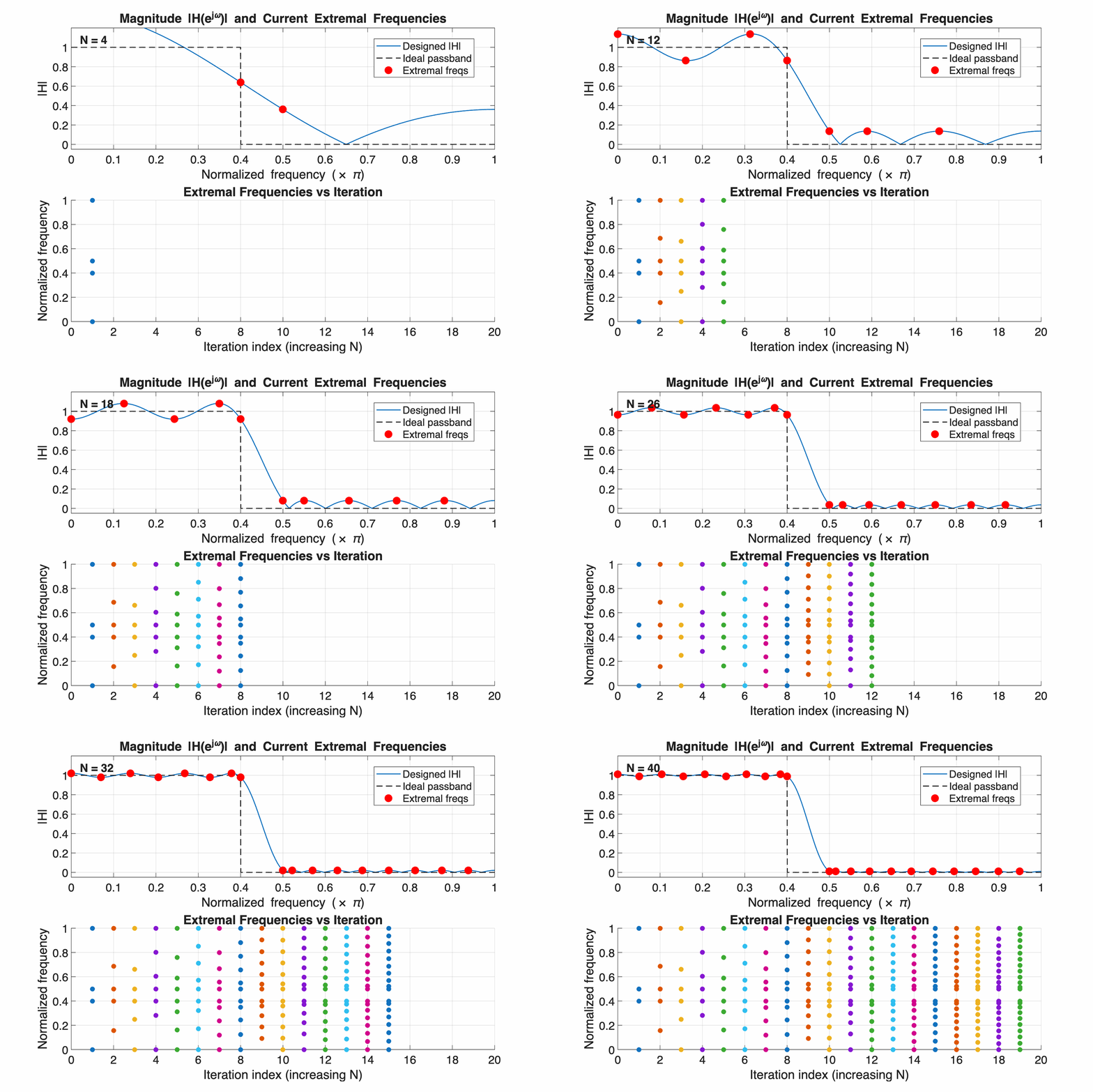
Steps 2–4 are hard to picture from a list, so it is worth watching them happen. firpm's third output returns the extremal set it settled on (res.fextr); running the design for \(N=4,6,8,\ldots,40\) and plotting that set each time turns the exchange into an animation, written straight out as a GIF.
Goal: watch the extremal frequencies multiply and settle as the order grows, and see the response go from a crude slope to a sharp equiripple edge without any change to the specification.
Animation_Parks_McClellan.m
MATLAB
%% Animation_Parks_McClellan.m - animate the extremal set as the order grows
% Animate extremal frequencies for increasing N and save as animated GIF.
Figure 7.2.d.Following the Parks–McClellan animation. The top panel shows the best equiripple response available at the current order; red markers identify the extremal frequencies where the weighted error reaches alternating positive and negative peaks. At a very low order, the filter has too few degrees of freedom to form a sharp edge. As the order increases, more extrema appear and the transition becomes narrower. The bottom panel keeps the extremal set from each design. The growing number of points agrees with the Alternation Theorem, and their concentration near the band edge shows where the approximation is most difficult. A printed page shows only the first frame; the on-screen animation shows the progression.
Weighting function for a two-band (passband/stopband) design:
This choice makes the weighted ripple identical in both bands: \(W(\omega_p)\delta_p=1\cdot\delta_p\) and \(W(\omega_s)\delta_s=(\delta_p/\delta_s)\delta_s=\delta_p\), so the algorithm's single equiripple level \(\delta\) (Eq. 7.7) enforces \(\delta_p\) in the passband and \(\delta_s\) in the stopband simultaneously.
A practical order estimate (Kaiser's formula, for a low-pass) gets the search started without guessing:
EXAMPLE 7.2 · Estimating the order of an equiripple low-pass
Design a minimax low-pass with \(A_p=0.5\,\text{dB}\), \(A_s=50\,\text{dB}\), passband edge \(f_p=0.15\), stopband edge \(f_s=0.20\) (normalized, \(f_s^{\text{sample}}=1\)). Estimate the order via Eq. (7.8) and state the design in MATLAB's terms.
Step 1 · Ripples. \(\delta_p=\dfrac{10^{A_p/20}-1}{10^{A_p/20}+1}=\dfrac{10^{0.025}-1}{10^{0.025}+1}\approx0.0288\), and \(\delta_s=10^{-A_s/20}=10^{-2.5}\approx0.00316\).
Step 3 · Order estimate. \(-10\log_{10}(\delta_p\delta_s)=-10\log_{10}(9.1\times10^{-5})\approx40.4\). By Eq. (7.8): \(M\approx\dfrac{40.4-13}{2.324(0.1\pi)}\approx\dfrac{27.4}{0.730}\approx37.6\Rightarrow M=38\) (round up).
Step 4 · In MATLAB. This is exactly what [M,fo,ao,w]=firpmord([0.15 0.20],[1 0],[0.0288 0.00316]) followed by b=firpm(M,fo,ao,w) automates — the Remez exchange (Section 7.2.2) then refines the guess to the true equiripple optimum, typically within a tap or two of this estimate.
MATLAB corner for Example 7.2
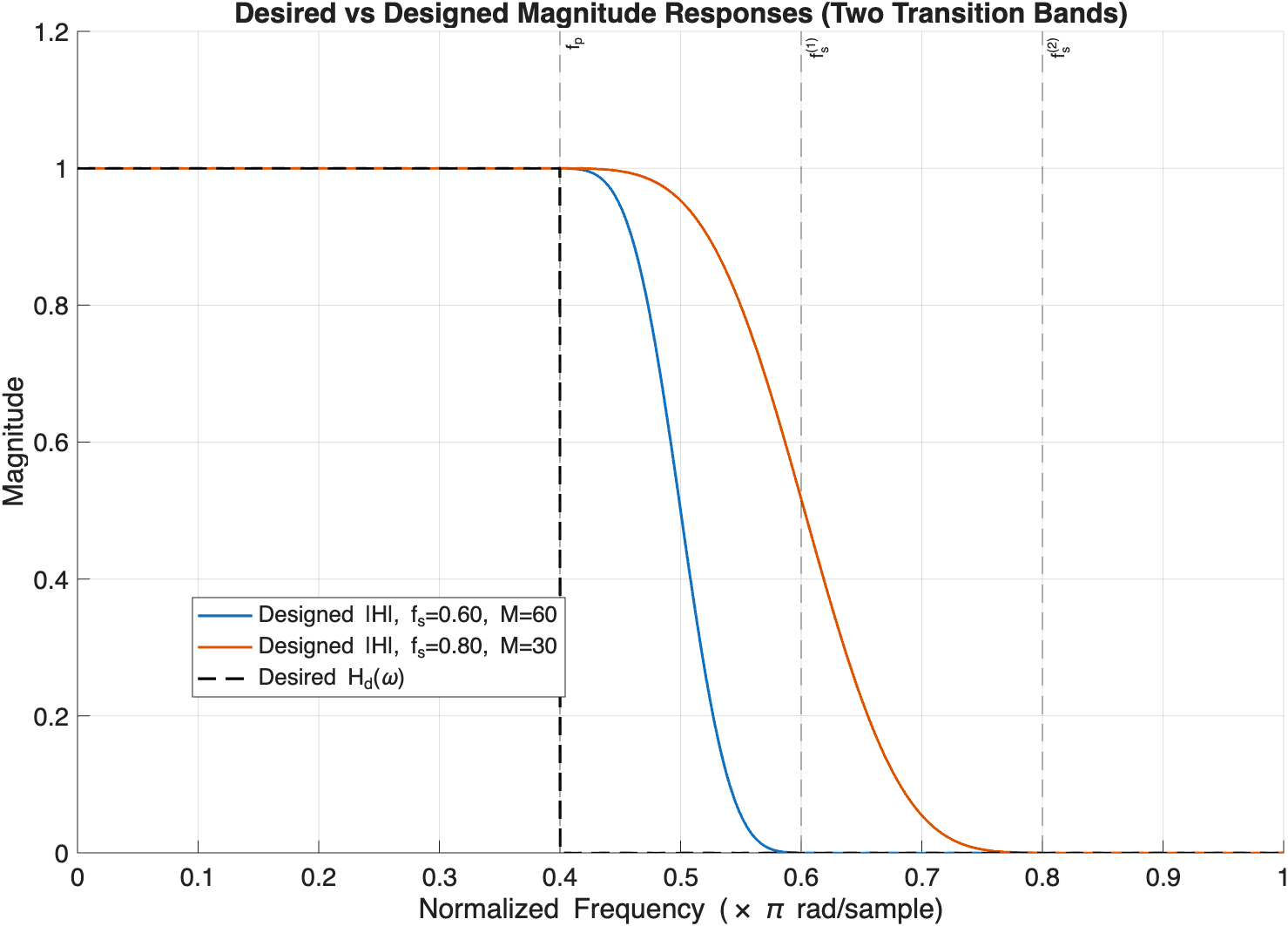
This script runs two firpm() designs at the same passband edge \(f_p=0.4\) but different stopband edges (\(f_s=0.6\) and \(0.8\)), so the order needed for a narrow transition can be read directly against a wide one. It plots the designed magnitudes against the ideal \(H_d\), zooms the passband to mark the extremal frequencies, and shows the impulse responses.
Goal: see the Alternation Theorem's equiripple signature in a real firpm() design (Figure 7.2.b, now for real), and confirm that halving the transition width roughly doubles the order Eq. (7.8) demands.
FIR_minimax.m
MATLAB
%% FIR_minimax.m - Remez/firpm designs at two transition widths
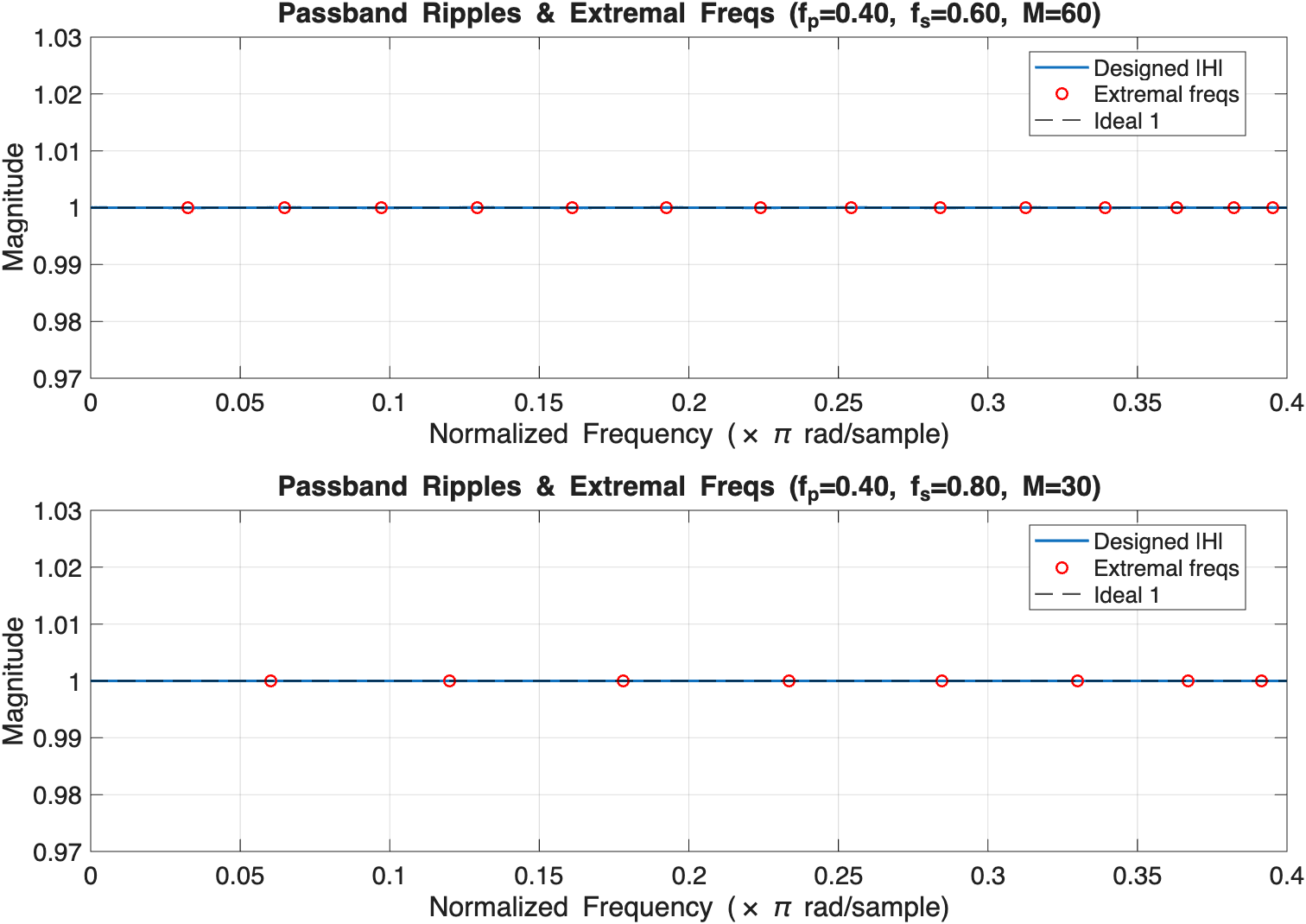
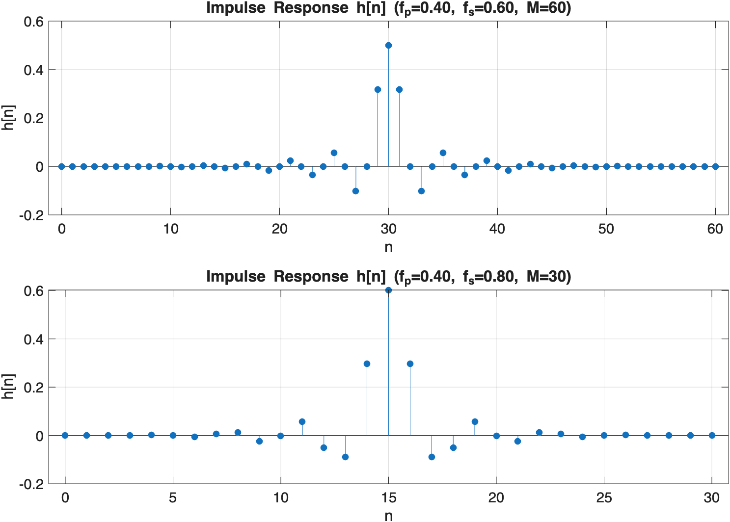
Figure 7.2.e.Effect of transition width on FIR order. Both firpm() designs use the same passband edge, \(f_p=0.4\), and the same error limits, \(\delta_p=\delta_s=0.01\). The design with \(f_s=0.8\) has a wide transition band and needs order \(M=30\). Moving the stopband edge to \(f_s=0.6\) halves the transition width, so the required order rises to about \(M=60\). The plots therefore confirm the inverse relationship in Eq. (7.8): a sharper transition needs a longer filter.Figure 7.2.f. The same two designs with the passband magnified to \(1\pm0.03\). The ripple is invisible at this scale because \(\delta=0.01\) was met with room to spare, but the extremal frequencies (red) are what matter: the Alternation Theorem requires at least \(M/2+2\) of them, and the order-60 design shows more than the order-30 one. Higher order buys more alternations, and more alternations are what allow a smaller \(\delta\).Figure 7.2.g. The coefficients themselves. Both are symmetric about their centre sample (\(n=30\) and \(n=15\)) with \(M\) even — i.e. Type I filters, exactly as Section 7.1 requires for a low-pass, and the group delay is the \(M/2\) samples visible as the position of the peak. Note also how much of the longer filter is nearly zero: order bought for a narrow transition is spent on a longer sinc tail, not on a different shape.
For fixed order and band edges, Parks–McClellan gives the linear-phase FIR filter with the smallest worst-case weighted error. Its disadvantage is that it requires an iterative numerical solver. The window method is more direct and easier to calculate by hand, but it usually needs more taps for the same specification.
7.3 The window method
The window method starts from the ideal infinite, non-causal impulse response and keeps only a finite section. By Parseval's theorem, minimizing mean-squared error in frequency is equivalent to minimizing the squared error between the desired and actual impulse-response coefficients:
If the practical filter must be zero outside \(0\le n\le M\), the minimum-error choice is to copy the ideal coefficients inside that interval and discard the rest. This is multiplication by a rectangular window. Replacing the abrupt rectangular cutoff with a smoother taper gives the general window method:
Multiplying by a window in time convolves the ideal response with the window spectrum \(W(e^{j\omega})\). The main-lobe width controls the filter's transition width, while the side-lobe level controls ripple and stopband attenuation. Reducing side lobes usually widens the main lobe, so every window makes a trade-off.
7.3.1 Why plain truncation is the MMSE solution
Take the ideal low-pass of Figure 7.3.a as the target. Its impulse response follows from the inverse DTFT, and it is a sinc: infinite in both directions, and decaying only as \(1/n\).
Now write the mean-squared error of Eq. (7.9) with the causal-FIR constraint \(h[n]=0\) for \(n\notin[0,M]\) made explicit, splitting the sum at the window boundary:
$$ \varepsilon^2=\sum_{n=-\infty}^{\infty}\big|h_d[n]-h[n]\big|^2=\underbrace{\sum_{n=0}^{M}\big|h_d[n]-h[n]\big|^2}_{\text{we control this}}\;+\;\underbrace{\sum_{n\notin[0,M]}\big|h_d[n]\big|^2}_{\text{fixed by }M\text{ alone}} $$
The second sum contains no design variable at all — it is the energy in the tails we are not allowed to keep. The first sum is a sum of independent non-negative terms, so it is minimised term by term, and its minimum is exactly zero, attained by \(h[n]=h_d[n]\) on \(0\le n\le M\). Hence:
So rectangular truncation is the optimal design in the mean-squared sense — no window, no cleverness, can do better on this criterion, and the residual error is just the discarded tail energy, which falls as \(M\) grows because the sinc tails decay.
Every window other than the rectangular one therefore has a worse mean-squared error. Windows are not there to reduce \(\varepsilon^2\); they are there to redistribute it.
7.3.2 Why the MMSE answer is still a bad filter
The catch is what the criterion measures. Squared error is an average over frequency, and the average is happy to hide a tall, narrow error at the band edge. Writing Eq. (7.10) out as the convolution integral,
the response at a chosen frequency depends on how much of the shifted window spectrum overlaps the ideal passband, as shown in Figures 7.3.c–7.3.e. For a rectangular window, increasing \(M\) narrows the oscillations but does not reduce the maximum overshoot near the discontinuity, which remains about 9%. This is the Gibbs phenomenon.
Windowing accepts a slightly larger \(\varepsilon^2\) in exchange for a much smaller peak error. Replacing the hard edges of \(w_R[n]\) with a smooth taper \(w[n]\) changes \(W\) in two coupled ways, and Section 7.4 is the catalog of that trade:
Side lobes → ripple
A taper that is continuous at the ends makes \(W\)'s side lobes decay faster, so less out-of-band area leaks in: passband and stopband ripple both fall. Gibbs is defeated.
Main lobe → transition
The same taper shortens the effective window length, widening \(W\)'s main lobe from \(4\pi/M\) to \(8\pi/M\) or \(12\pi/M\): the transition band widens for the same order.
Figure 7.3.a. Where the window method starts: the ideal \(A_d(\omega)\) of Eq. (7.9) is a brick wall of height 1 out to \(\omega_c\), periodic in \(\omega_s\). Its impulse response is an infinite, non-causal sinc — which is exactly why it has to be truncated.Figure 7.3.b. The window's own transform \(W(e^{j\omega})\), and the whole trade in one picture: the main-lobe width becomes the realised transition bandwidth, and the side-lobe height becomes passband and stopband ripple. Every window choice moves these two in opposite directions.
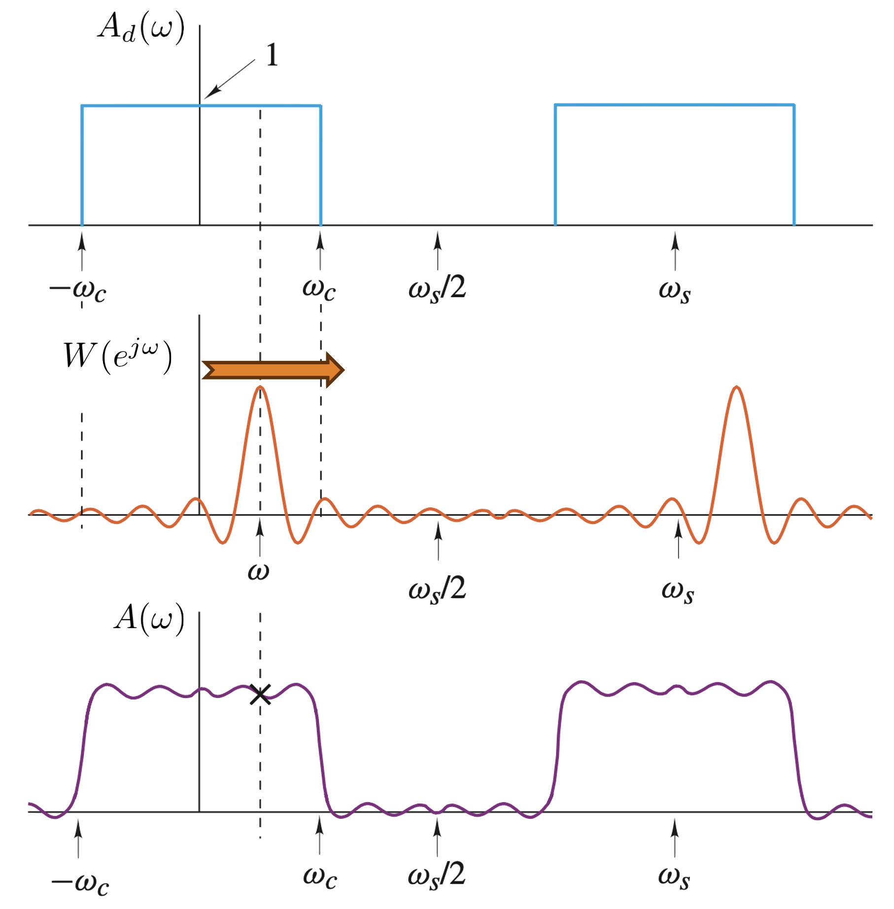
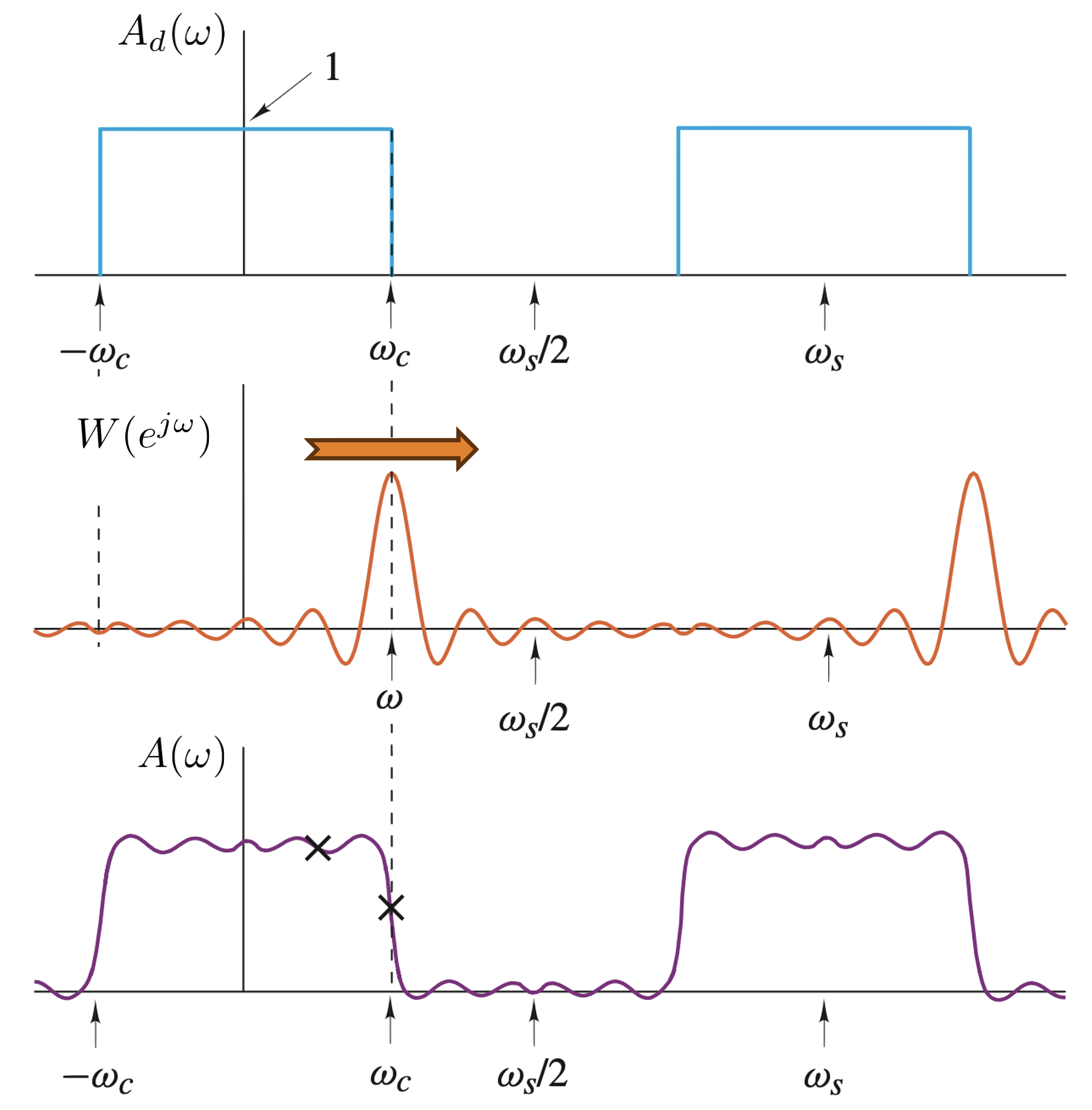
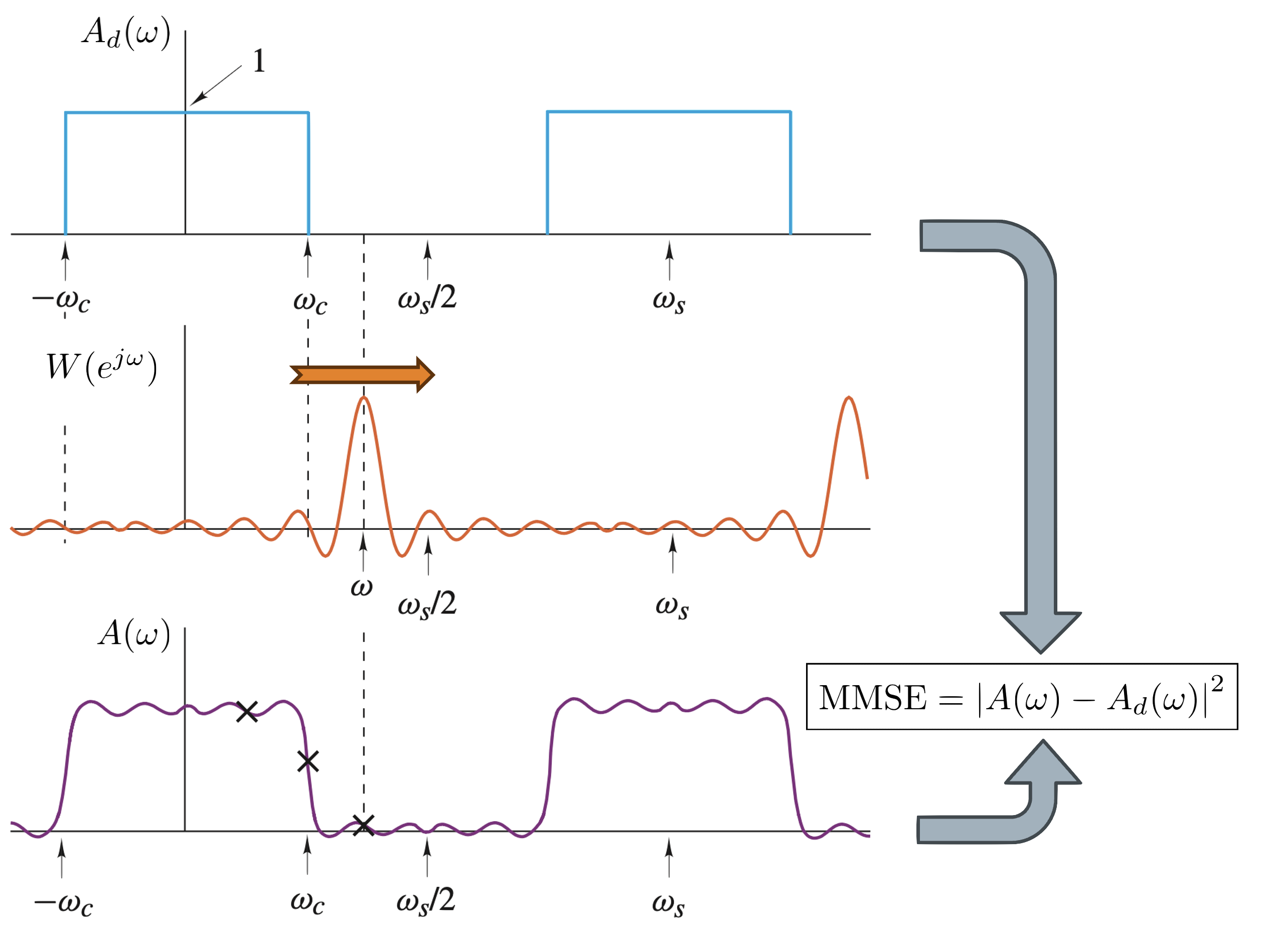
Figures 7.3.c–7.3.e show the same convolution at three positions: inside the passband, at the cutoff and in the stopband. In each case, the output is determined by how much of the shifted window spectrum overlaps the ideal passband.
Figure 7.3.c. Eq. (7.10) evaluated deep inside the passband. Sliding \(W(e^{j\omega})\) to a frequency well below \(\omega_c\) (orange arrow), the main lobe is entirely enclosed by the ideal band, so the integral collects the whole main lobe and \(A(\omega)\approx1\) — the small wobble that remains is what the side lobes outside the band contribute.Figure 7.3.d. The same product at \(\omega=\omega_c\). Now the main lobe straddles the edge, so only about half of it lies inside the band and \(A(\omega_c)\approx0.5\). The response therefore falls over the frequency span it takes the main lobe to cross the edge: the main-lobe width is the transition width.Figure 7.3.e. Past the edge only side lobes overlap the ideal band, and what they leak is the stopband ripple. The MMSE box states what Eq. (7.9) is actually minimising, \(|A(\omega)-A_d(\omega)|^2\) — and makes plain that windowing controls this error by reshaping \(W\), never by removing it.
The main design choice is therefore the taper. Stronger tapering lowers side lobes and improves stopband attenuation, but widens the main lobe and requires more taps for the same transition width.
7.4 Window catalog and order estimates
The next sections compare four fixed windows and the adjustable Kaiser window. Each is shown in time and frequency because the taper shape controls implementation, while its spectrum controls transition width and ripple.
Hann, Hamming and Blackman windows are sums of cosine terms. In frequency, each cosine creates shifted copies of the rectangular-window spectrum. Their weights are selected so that side lobes cancel. The same combination also merges several main lobes into a wider one, which explains the basic trade-off.
MATLAB corner
One loop builds all five windows at \(M=51\) and plots each one twice: the taper \(w[n]\) itself, and \(20\log_{10}|W(e^{j\omega})|\) normalised to its peak. A second block sweeps \(\beta\) for the Kaiser family. Every figure in the rest of this section is an output of this script.
Goal: measure the main-lobe width and side-lobe floor of each window in the catalog, and confirm the two move in opposite directions exactly as Section 7.3.2 predicts.
FIR_windows.m
MATLAB
%% FIR_windows.m - separate window plots: time vs frequency
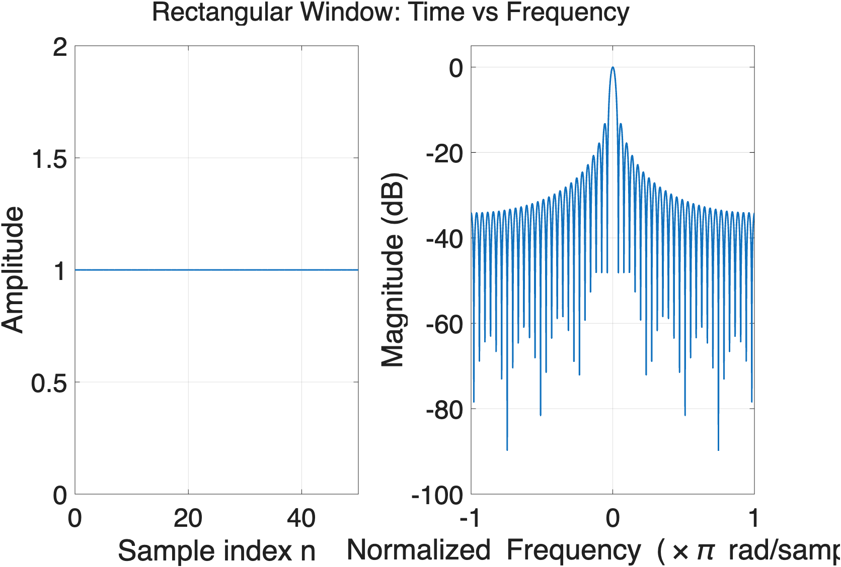
The Dirichlet kernel, and the parent of every entry below. Its main lobe is the narrowest achievable for \(M+1\) taps, but the side lobes fall off only as \(1/\omega\) — the abrupt end of the window is a step, and a step has a slowly decaying spectrum.
main lobe \(4\pi/M\)first side lobe \(-13\,\text{dB}\)decay \(1/\omega\)\(K=4\)
Figure 7.4.a. The rectangular window — plain truncation, in time (left) and dB (right). It has the narrowest main lobe of any window, hence the sharpest transition for a given order, and the worst side lobes: the first sits at \(-13\,\text{dB}\) and the floor barely falls with frequency, so no amount of extra taps buys stopband depth.
Three Dirichlet kernels, the outer two shifted by exactly one main-lobe half-width and inverted. Where the centre kernel's first side lobe is positive the shifted ones are negative, so they cancel — and the window now reaches zero with zero slope, so the decay steepens to \(1/\omega^3\). The price is that the three main lobes merge into one twice as wide.
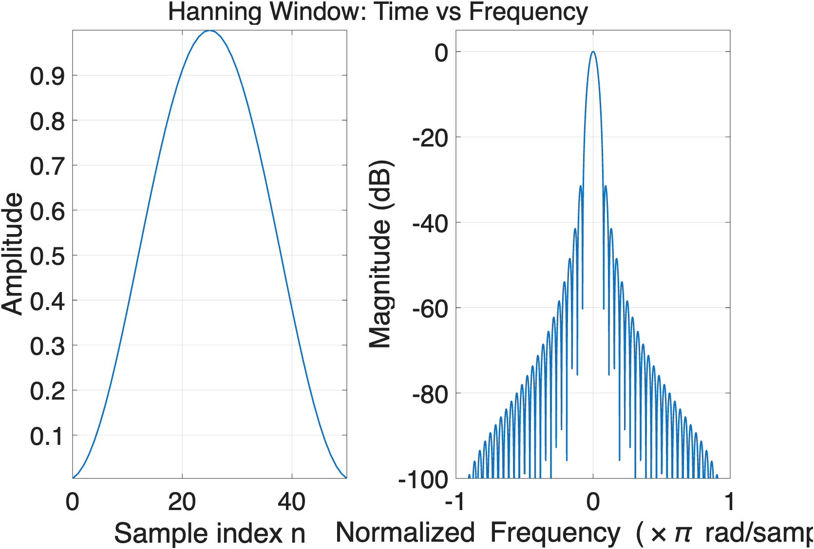
main lobe \(8\pi/M\)first side lobe \(-31\,\text{dB}\)decay \(1/\omega^3\)\(K=8\)
Figure 7.4.b. The Hann raised cosine goes smoothly to zero at both ends. That single change doubles the main-lobe width but drops the first side lobe to \(-31\,\text{dB}\) and makes the rest decay steeply — the Eq. (7.10) trade in its simplest form.
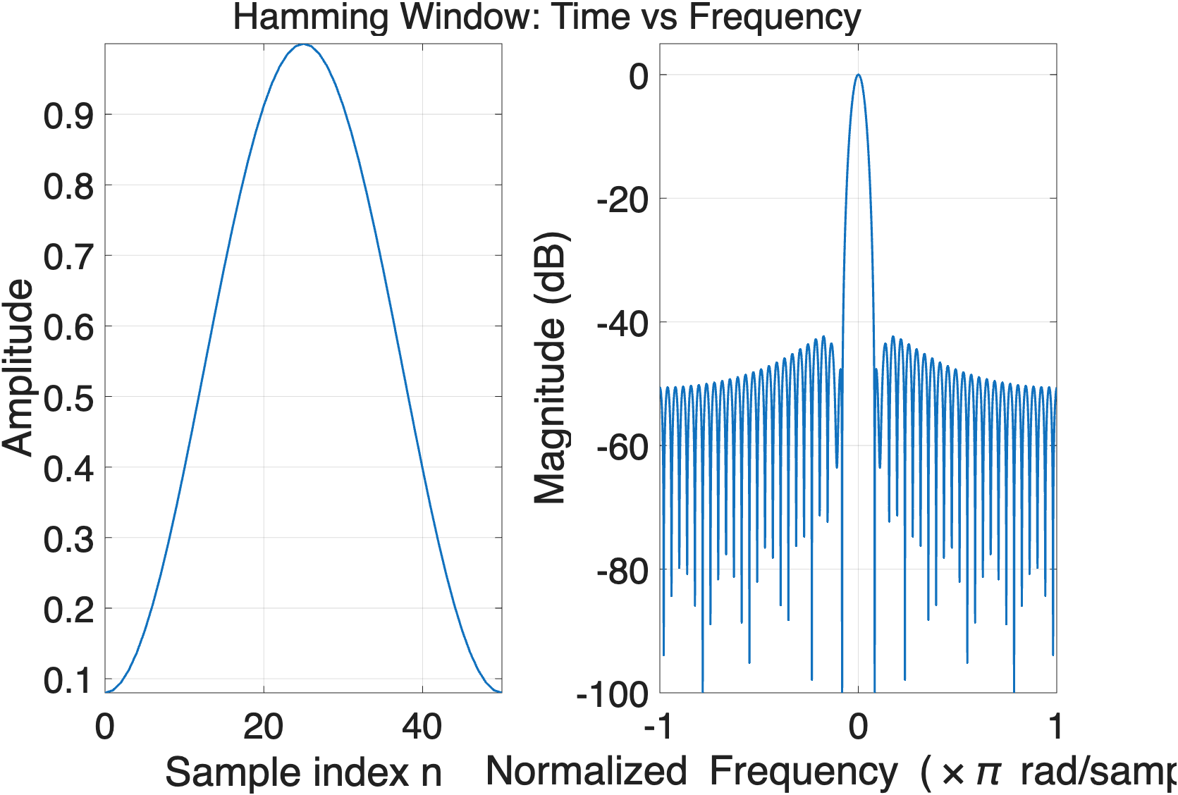
The same three-kernel sum with the weights re-tuned: \(0.54/0.46\) instead of \(0.5/0.5\) is chosen so the cancellation lands on the largest remaining side lobe rather than being spread evenly. The floor flattens near \(-41\,\text{dB}\) instead of decaying, and the main lobe is unchanged from Hann — 10 dB for free.
main lobe \(8\pi/M\)first side lobe \(-41\,\text{dB}\)flat floor\(K=8\)
Figure 7.4.c.Hamming keeps Hann's main-lobe width but adds a small pedestal, which cancels the largest side lobe and flattens the floor to about \(-41\,\text{dB}\). It is the usual default when 40–50 dB of stopband is enough.
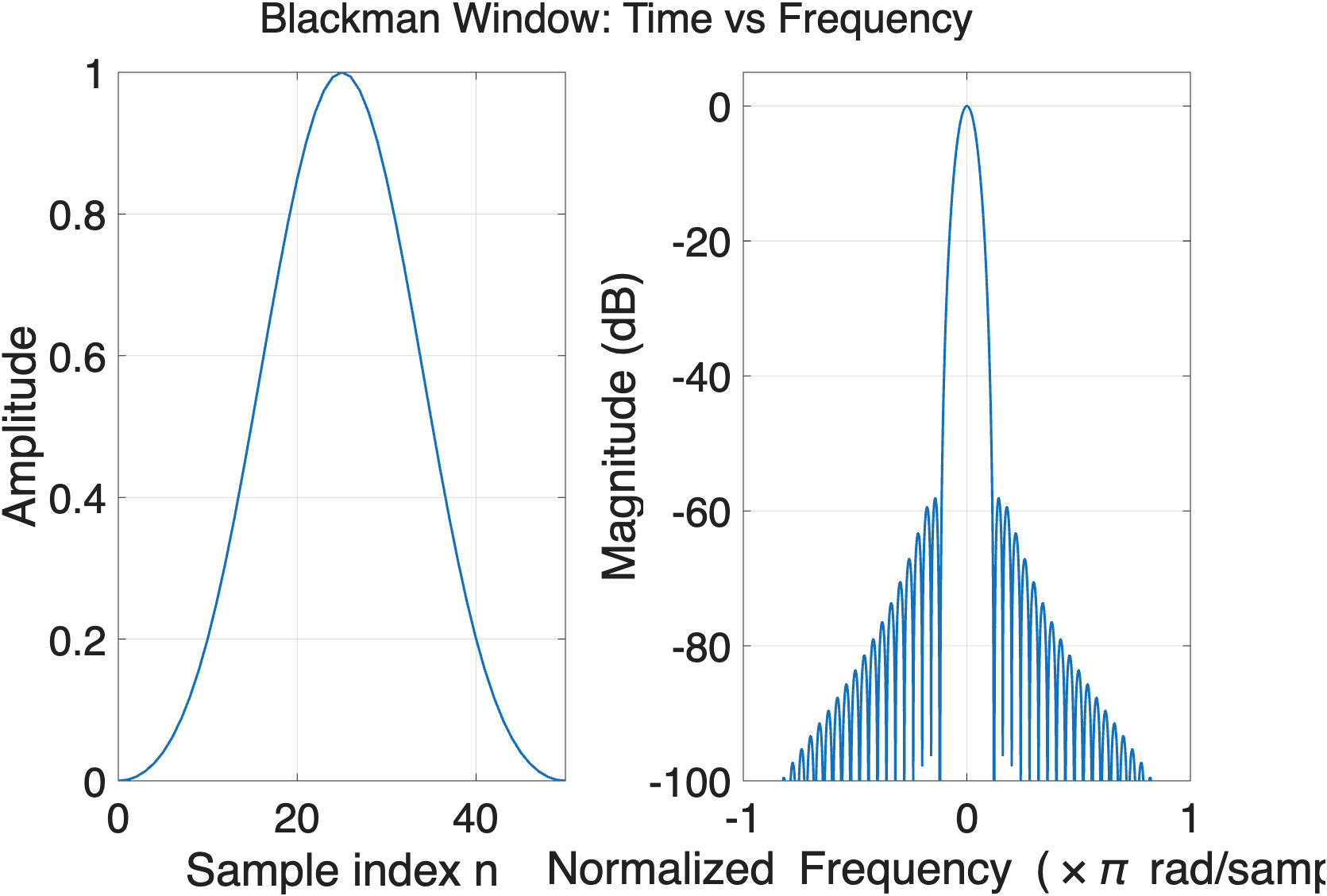
A second harmonic adds two more shifted kernels, at \(\pm4\pi/M\), giving five terms to cancel with instead of three: the floor drops to \(-57\,\text{dB}\). Five merging main lobes is a \(12\pi/M\) main lobe — three times the rectangular width, i.e. three times the taps for the same transition.
main lobe \(12\pi/M\)first side lobe \(-57\,\text{dB}\)5 kernels\(K=12\)
Figure 7.4.d.Blackman adds a third cosine term, reaching about \(-57\,\text{dB}\) with a main lobe three times the rectangular width — i.e. three times the taps for the same transition. This is the window behind Example 7.3's 60 dB design.
Fixed windows offer only a few attenuation choices. For example, a 47 dB requirement is too demanding for Hamming at about 41 dB, while Blackman at about 57 dB provides more attenuation—and usually more taps—than required. A tunable window can match the target more closely.
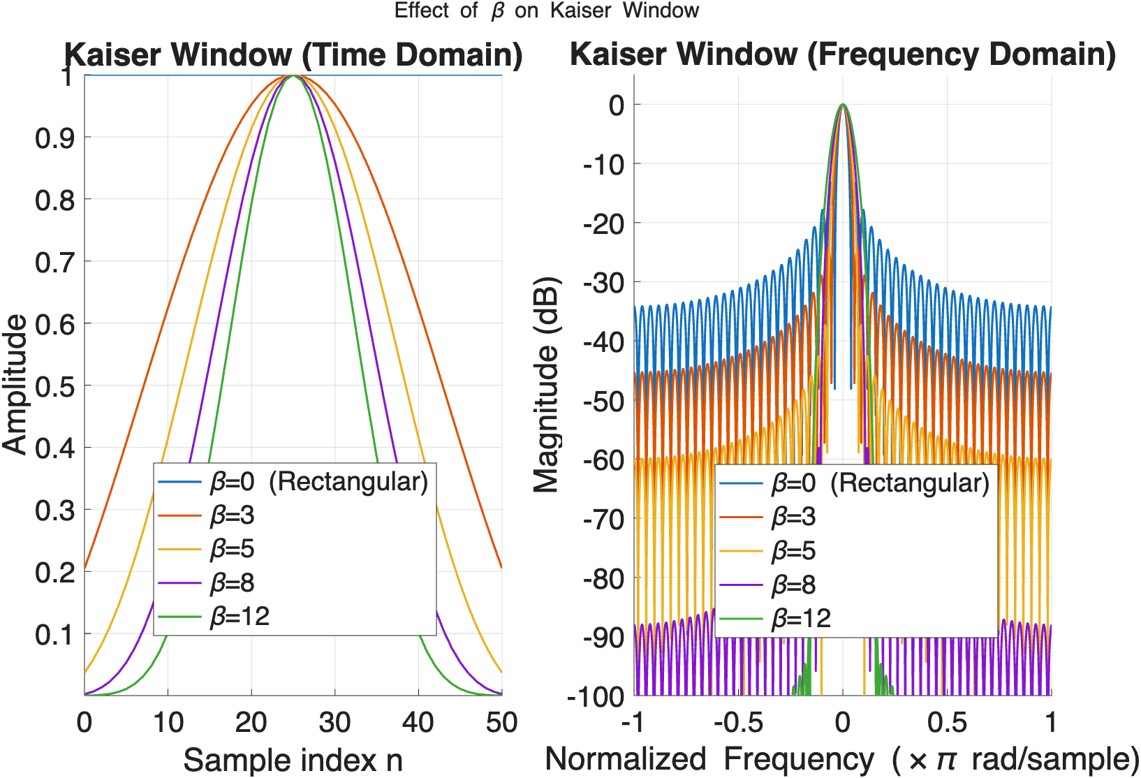
Not a cosine sum at all: \(I_0\) is the zeroth-order modified Bessel function, and the transform is the \(\sinh\) form above inside the main lobe — past \(|\omega|=2\beta/M\) the radicand turns negative and the \(\sinh\) becomes an ordinary \(\sin\), i.e. side lobes. It nearly maximises main-lobe energy for a given side-lobe level, and \(\beta\) moves along that optimum continuously: \(\beta=0\) returns \(w_R[n]\), \(\beta\approx5\) sits near Hamming, \(\beta\approx8.5\) near Blackman. Eqs. (7.12)–(7.13) invert it for design.
main lobe \(\approx 4\sqrt{\pi^2+\beta^2}/M\)side lobe set by \(\beta\)tunablesee Eq. (7.13)
Figure 7.4.e. Why Kaiser replaces the table: \(\beta\) sweeps the same trade continuously. \(\beta=0\) is exactly the rectangular window of Figure 7.4.a; raising \(\beta\) tapers harder and drops the side-lobe floor (roughly \(-35,-46,-60,-90\,\text{dB}\) for \(\beta=0,3,5,8\)) while widening the main lobe. Eq. (7.11) is this family solved backwards: state the \(A_s\) you need and it returns \(\beta\) and the order.
Window
Sidelobe
Mainlobe
\(K\)
Use
Rectangular
−13 dB
\(4\pi/M\)
4
Max resolution, leaky
Hann
−31 dB
\(8\pi/M\)
8
Lower ripple than rect.
Hamming
−41 dB
\(8\pi/M\)
8
Popular default
Blackman
−57 dB
\(12\pi/M\)
12
Strong stopband
Kaiser (\(\beta\))
tunable
tunable
—
Best all-round
The fixed-window order estimate reads the transition width straight off the table:
$$ M\approx\frac{K\pi}{\Delta\omega}-1 $$
(7.11)
Kaiser's window replaces the fixed catalog with one continuously tunable shape, letting a single parameter \(\beta\) buy exactly the stopband attenuation needed without over-paying in order:
$$ w_K[n]=\frac{I_0\!\Big(\beta\sqrt{1-(2n/M-1)^2}\Big)}{I_0(\beta)},\qquad 0\le n\le M $$
(7.12)
The shape parameter itself follows from the required stopband attenuation \(A_s\) in dB:
with order estimate \(M\approx\dfrac{A_s-8}{2.285\,\Delta\omega}\), consistently a bit lower than Eq. (7.11) would give the corresponding fixed window for the same attenuation, because Kaiser's taper is tuned exactly to the target instead of over- or under-shooting it.
EXAMPLE 7.3 · A narrow-transition low-pass with a fixed window
Design a low-pass filter with \(A_p=0.1\,\text{dB}\), \(A_s=60\,\text{dB}\), passband \(0\le|f|\le0.24\), stopband \(0.26\le|f|\le0.5\) (normalized). Pick the best fixed window from Table 7.4's catalog and state the filter's order, type, and group delay.
Step 2 · Window choice. Need at least 60 dB attenuation; Table 7.4 gives Hann 44 dB, Hamming ~53 dB, Blackman ~74 dB — only Blackman clears 60 dB.
Step 3 · Order. By Eq. (7.11), \(K=12\): \(M\approx\dfrac{12\pi}{0.04\pi}-1=299\). \(M\) even ⇒ Type I, length \(L=300\), group delay \(\tau=M/2=149.5\).
Step 4 · Ideal response. Cutoff at the transition centre: \(f_c=\tfrac{0.24+0.26}{2}=0.25\), \(\omega_c=0.5\pi\), so \(h_d[n]=\dfrac{\sin(\omega_c(n-M/2))}{\pi(n-M/2)}\) (with \(h_d[M/2]=\omega_c/\pi=0.5\)), and the final filter is \(h[n]=h_d[n]\,w_{\text{Blackman}}[n]\).
MATLAB corner for Example 7.3
This script builds Example 7.3's Blackman-windowed filter directly from the ideal sinc and checks the actual passband/stopband ripple against the \(A_p,A_s\) targets.
Goal: confirm the \(M=299\) Blackman design meets \(A_p=0.1\), \(A_s=60\,\text{dB}\), and show the characteristic tapering ripple (not equiripple, unlike Figure 7.2.e).
window_lpf_design.m
MATLAB
%% window_lpf_design.m - Example 7.3's Blackman-windowed LPF (Eq. 7.10-7.11)
M = 299; n = (0:M)';
fc = 0.25; wc = 2*pi*fc;
hd = sin(wc*(n-M/2)) ./ (pi*(n-M/2)); % ideal sinc, Eq. (7.9)
hd(n==M/2) = wc/pi; % L'Hopital limit at the centre tap
Figure 7.4.f.Reading the Blackman-window design. The order-299 filter reaches the required 60 dB stopband attenuation. Its largest side lobe occurs near the band edge, and the later side lobes become progressively smaller. This is the characteristic shape imposed by the Blackman window. It differs from the Parks–McClellan result in Figure 7.2.e, where the error peaks have nearly equal height across each constrained band. The window design is straightforward, but it does not distribute the available error as efficiently as an equiripple design.
EXAMPLE 7.4 · The same low-pass, redesigned with a Kaiser window
Repeat Example 7.3's specification (\(A_s=60\,\text{dB}\), \(\Delta\omega=0.04\pi\)) using the Kaiser window instead, and compare the resulting order to Blackman's \(M=299\).
Step 1 · Order. \(M\approx\dfrac{A_s-8}{2.285\,\Delta\omega}=\dfrac{60-8}{2.285(0.04\pi)}\approx181\). Round up to an even order for Type I: \(\boxed{M=182}\), \(L=183\), \(\tau=91\).
Step 2 · Shape parameter. Since \(A_s=60>50\), Eq. (7.13)'s top case applies: \(\beta\approx0.1102(60-8.7)=0.1102(51.3)\approx\boxed{5.65}\).
Step 3 · Comparison. Kaiser reaches the same 60 dB, 0.02-wide transition in \(M=182\) versus Blackman's \(M=299\) — 39% fewer taps, because Blackman's fixed \(-57\,\text{dB}\) design over-delivers stopband depth it was not asked for, while Kaiser's \(\beta\) is tuned to exactly 60 dB and no more.
MATLAB corner for Example 7.4
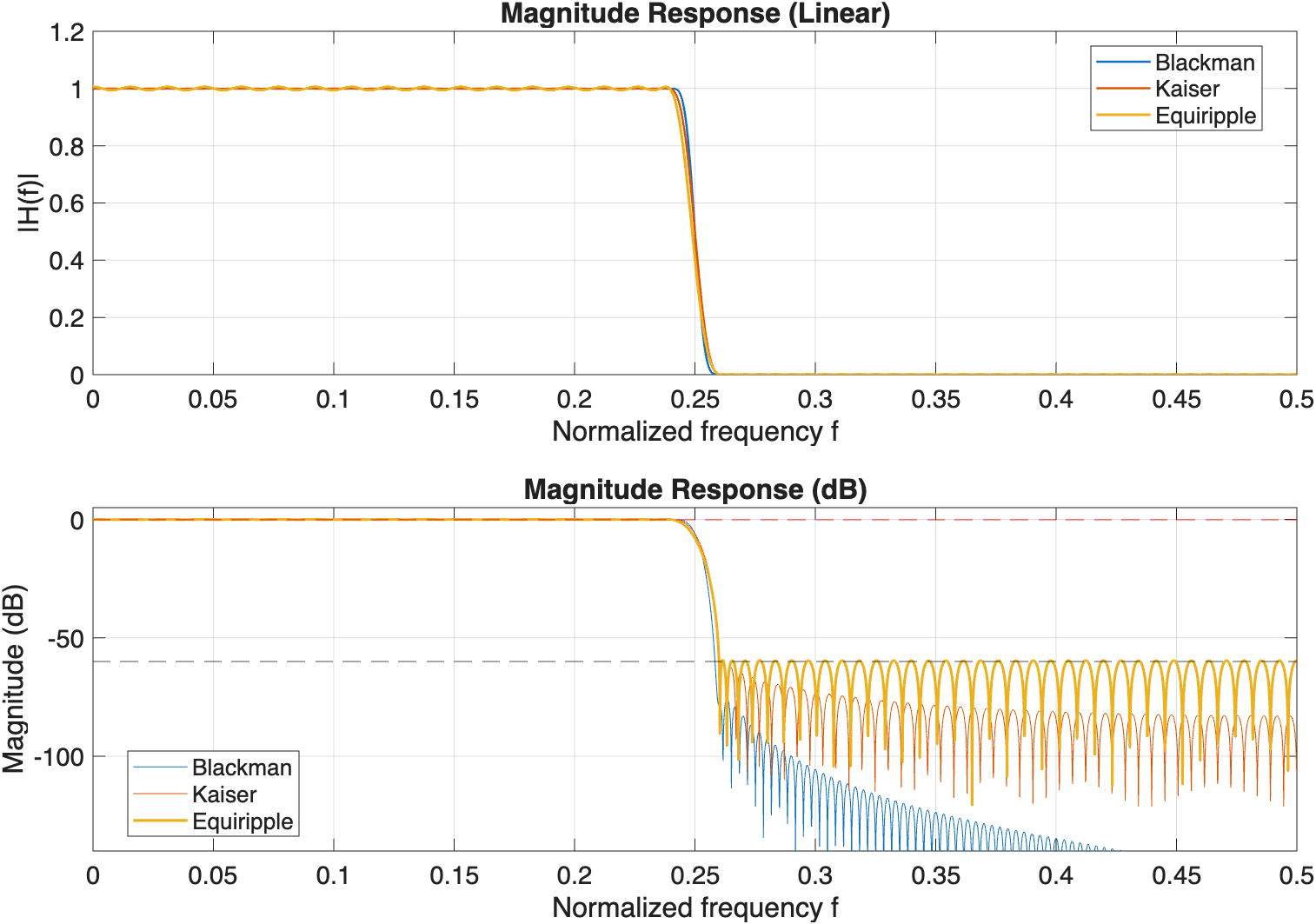
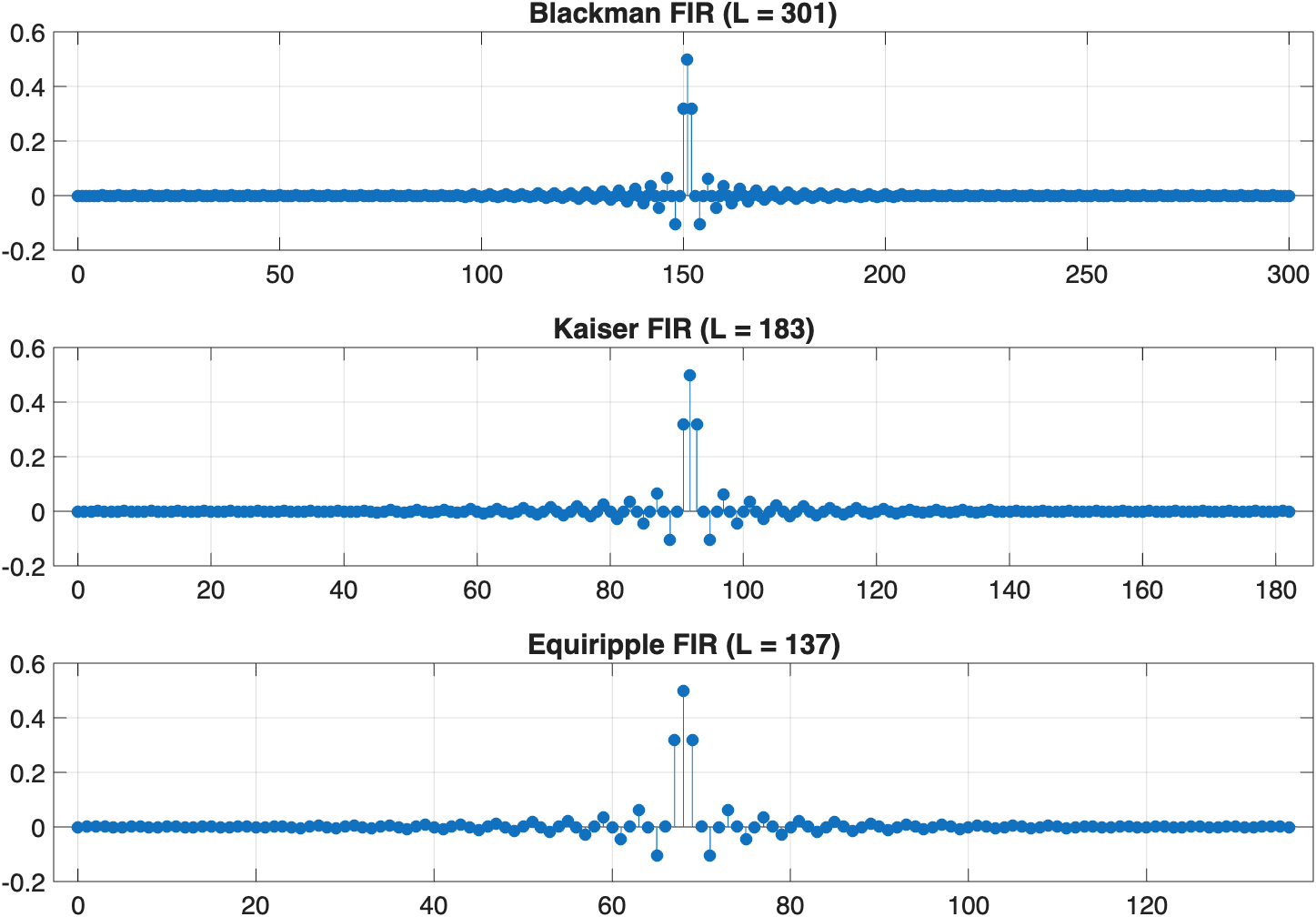
This script designs Example 7.3's specification three ways at once — Blackman, Kaiser, and Parks–McClellan — from the same ideal sinc, and prints a table of order, length and group delay for each. It is the whole lecture in one file: the same target, reached by both methods of the comparison table above.
Goal: confirm the Kaiser design (\(M=182,\beta=5.65\)) meets the same 60 dB target as the Blackman design (\(M=299\)) with far fewer taps.
FIR_exmp_1.m
MATLAB
%% FIR_exmp_1.m - FIR lowpass filter comparison
% Blackman vs Kaiser vs Equiripple (Parks–McClellan)
Figure 7.4.g.Three methods for the same low-pass specification. On the linear-scale plot, the equiripple, Kaiser and Blackman responses are almost indistinguishable because all three meet the passband requirement and use the same band edge at \(f=0.25\). The dB plot reveals how they use the stopband tolerance. The equiripple design keeps its largest errors close to \(-60\,\text{dB}\) throughout the stopband, using the allowed error evenly. The Kaiser and Blackman side lobes fall below \(-80\,\text{dB}\) away from the edge. That extra attenuation was not required and generally costs additional taps.Figure 7.4.h.Coefficient count and computational cost. The Blackman design uses 301 taps, the Kaiser design uses 183, and the Parks–McClellan design uses 137. All three meet the same specification, so the shorter minimax filter requires fewer multiplications per output sample and has less delay. Each impulse response is symmetric about its centre sample, confirming an exact-linear-phase Type I filter. The methods differ in length, not in the linear-phase property.
An ideal band-pass impulse response is the difference between two ideal low-pass responses. The same windowing procedure therefore applies. The important extra step is to calculate both transition widths; the narrower transition determines the required order.
EXAMPLE 7.5 · A band-pass design, Hann against Kaiser
Design a band-pass filter with stopband edges \(f_{1s}=0.125\), \(f_{2s}=0.40\) and passband \(0.175\le f\le0.30\) (normalized, Nyquist \(=0.5\)), with \(\delta_p=0.05\) and \(\delta_s=0.01\). Give the order and type using the Hann window, then again using Kaiser, and say which transition band decides the answer.
Step 1 · Specifications in dB. \(A_p=20\log_{10}\dfrac{1+\delta_p}{1-\delta_p}\approx0.87\,\text{dB}\) and \(A_s=-20\log_{10}\delta_s=40\,\text{dB}\).
Step 2 · The binding transition. The lower transition is \(0.175-0.125=0.05\), the upper is \(0.40-0.30=0.10\). The window smears both edges by the same main-lobe width, so the narrower one governs: \(\Delta f=0.05\Rightarrow\Delta\omega=0.1\pi\).
Step 3 · Hann. Hann gives \(\approx44\,\text{dB}\), clearing the 40 dB target. With \(K=8\) from the catalog, Eq. (7.11) gives \(M\approx8\pi/0.1\pi-1=79\) — odd, so a Type II filter (even symmetry, \(M\) odd), group delay \(M/2=39.5\) samples. A Type II forced zero sits at \(z=-1\), which is harmless here: \(\omega=\pi\) is deep in the stopband.
Step 4 · Kaiser. \(M\approx\dfrac{A_s-8}{2.285\,\Delta\omega}=\dfrac{40-8}{2.285(0.1\pi)}\approx45\), rounded up to an even order for Type I, with \(\beta\) from Eq. (7.13)'s middle case: \(\beta=0.5842(19)^{0.4}+0.07886(19)\approx3.40\). Group delay \(\approx23\) samples.
Kaiser reaches the same 40 dB with roughly 40% fewer taps (\(M=46\) against \(79\)), because Hann over-delivers (44 dB where 40 was asked) while \(\beta\) is tuned to the target exactly — the same over-payment Example 7.4 found at 60 dB, and the reason Kaiser is the default.
MATLAB corner
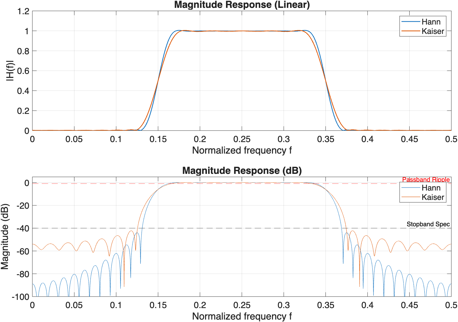
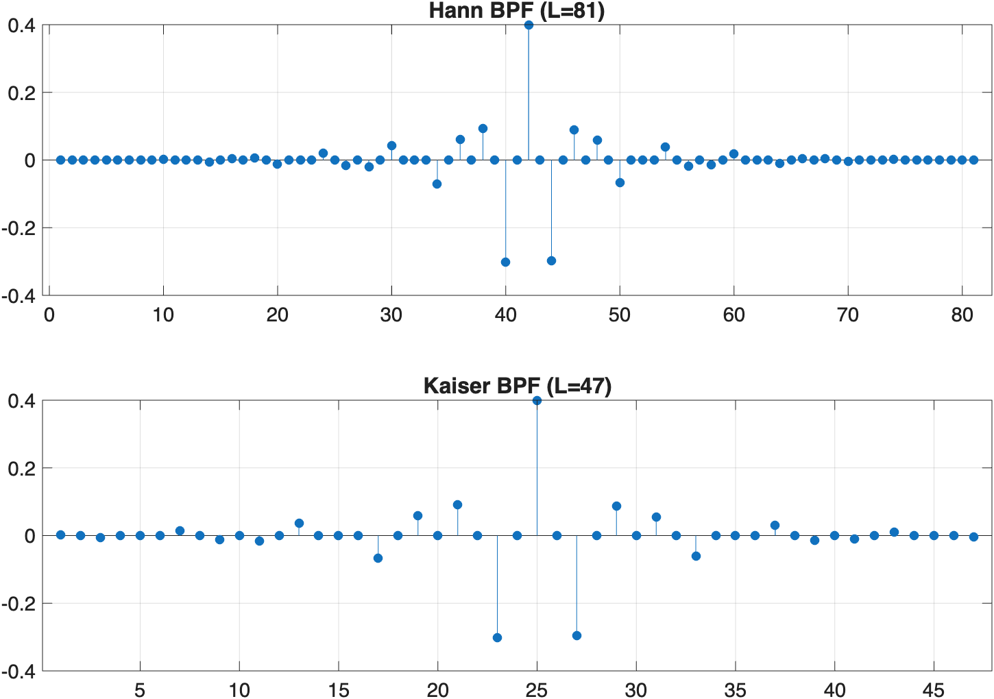
This script builds Example 7.5 both ways: it forms the ideal band-pass as a difference of two low-pass sincs, applies the Hann and Kaiser windows of the same centred slice, and prints the order, group delay and \(\beta\) for each.
Goal: confirm both designs clear the 40 dB stopband and 0.87 dB passband specs, and that Kaiser does it with roughly 40% fewer taps than Hann.
Figure 7.4.i.Hann and Kaiser band-pass designs compared. Both responses remain inside the \(0.87\,\text{dB}\) passband limit and below the \(-40\,\text{dB}\) stopband limit. The lower transition is narrower than the upper one, so it determines the required order and produces the sharper edge. The windows differ mainly in the stopband shape. The Hann side lobes decrease with distance from the passband and fall below \(-80\,\text{dB}\) near DC. The Kaiser side lobes remain near \(-55\,\text{dB}\). That floor is higher, but it still satisfies the specification; the adjustable Kaiser parameter provides direct control over this trade-off.Figure 7.4.j.Why the Kaiser design is shorter. The Hann design needs 81 taps, while the adjustable Kaiser window meets the same limits with 47 taps, a reduction of about 40%. Both coefficient sequences contain the oscillating ideal band-pass impulse response multiplied by a smooth taper. Both are symmetric, so both have exact linear phase. The plotted length also identifies the linear-phase type: an odd number of taps means even order and Type I; an even number of taps means odd order and Type II.
7.5 The window design recipe
A practical design starts with passband ripple and stopband attenuation in decibels, together with frequency edges. The following steps convert those requirements into a window, filter length, cutoff and coefficient sequence.
7.5.1 Reading the specification
Window formulas use linear ripple tolerances, so first convert the passband ripple \(A_p\) and stopband attenuation \(A_s\) from decibels into \(\delta_p\) and \(\delta_s\):
The frequency specs are the two band edges. The window smears the ideal brick wall symmetrically about its own centre (Figure 7.3.d), so the ideal cutoff is placed at the middle of the transition band, and the width of that band is what sets the order:
$$ f_c=\tfrac{1}{2}(f_p+f_s),\qquad \Delta f=f_s-f_p,\qquad \omega_c=2\pi f_c,\qquad \Delta\omega=2\pi\Delta f $$
(7.15)
Unlike minimax design, a window does not independently control passband and stopband ripple. The same window spectrum affects both bands, so the design must satisfy the tighter of \(\delta_p\) and \(\delta_s\). The other band will usually perform better than required.
and, if the design has more than one transition band (a band-pass or band-stop), the order is set by the narrowest of them for the same reason — one main lobe has to fit through the tightest gap.
Figure 7.5.a. The specification, drawn. Everything Eqs. (7.14)–(7.16) manipulate is visible here: the passband corridor \(1-\delta_p\le|H(f)|\le1+\delta_p\) out to \(f_p\), the stopband ceiling \(|H(f)|\le\delta_s\) from \(f_s\) to Nyquist, the transition band \(\Delta f=f_s-f_p\) that the window's main lobe has to fit inside, and the ideal cutoff \(f_c=\tfrac12(f_p+f_s)\) placed at its centre. The two dB brackets on the left are the same two constraints as the designer states them, \(A_p\) peak-to-peak across the passband corridor and \(A_s\) down to the stopband ceiling.
Two numbers come out of the specification and nothing else matters: \(A\) picks the window shape, \(\Delta\omega\) picks the window length. They are independent knobs, which is exactly why the method needs no iteration.
7.5.2 The recipe, with a fixed window
For a fixed window, use the required attenuation to choose the window and its constant \(K\). Use the narrowest transition width in Eq. (7.11) to estimate \(M\), place \(\omega_c\) at the transition centre, calculate the ideal sinc and multiply by the window.
Figure 7.5.b. The window design recipe with a fixed window, in six numbered steps — the same six as the checklist at the end of this section, with steps 1 and 3 reading their inputs straight off Figure 7.5.a. Amplitude specs set the shape through the worst-case ripple \(A\) of Eq. (7.16); frequency specs set the length through Eq. (7.11), using the \(K\) belonging to the shape already chosen. The two meet in \(w[n]\), which multiplies the ideal sinc evaluated at the transition-centre cutoff \(\omega_c\). Nothing feeds back: the only correction is rounding \(L\) so the resulting type can realise the response wanted.
7.5.3 The same recipe with a Kaiser window
For a Kaiser design, use the required attenuation to calculate the shape parameter \(\beta\) and use the Kaiser order estimate. The remaining steps—ideal sinc, delay, multiplication and verification—are unchanged.
Figure 7.5.c. The Kaiser variant, numbered the same way. Only steps 2 and 4 change: the table lookup is replaced by Eq. (7.13), which turns the required attenuation \(A\) straight into \(\beta\), and the order estimate becomes Kaiser's own — both continuous in \(A\), which is why the design pays for exactly the attenuation asked for and no more (Examples 7.4 and 7.5).
7.5.4 Adjusting the length for the type
The order estimate must be rounded up to an integer. Its parity determines the FIR type and therefore any forced zeros. Choose an even or odd order that is compatible with the required response.
Low-pass
Type I or II. Either parity works — the forced zero at \(z=-1\) sits deep in the stopband.
High-pass
Type I only: \(M\) must be even, or the \(z=-1\) zero kills the passband at \(\omega=\pi\).
Band-pass
Type I or II (Example 7.5 uses both). Order set by the narrower of the two transitions.
Band-stop
Type I only: it must pass both DC and \(\omega=\pi\), so no forced zero is tolerable.
Figures 7.5.b and 7.5.c summarise the window method. (1) Convert \(A_p\) and \(A_s\) to the linear tolerances \(\delta_p\) and \(\delta_s\). (2) Use the stricter tolerance to choose a fixed window or the Kaiser parameter \(\beta\). (3) Place \(\omega_c\) at the centre of the transition and find the narrowest transition width \(\Delta\omega\). (4) Estimate the required length and adjust its parity for the FIR type. (5) calculate the window \(w[n]\). (6) multiply it by the shifted ideal sinc to obtain \(h[n]\), then verify the result. The length formulas are estimates, so add two taps and check again if a limit is missed slightly.
Example
Spec
\(A\)
Shape
\(\Delta\omega\)
\(M\)
7.3
LPF, 0.24/0.26
60 dB
Blackman
\(0.04\pi\)
299
7.4
same spec
60 dB
Kaiser \(\beta=5.65\)
\(0.04\pi\)
182
7.5
BPF, 0.125–0.40
40 dB
Hann / Kaiser \(\beta=3.40\)
\(0.1\pi\)
79 / 46
Three specifications, one procedure, and the only judgement anywhere in it is step 2 — which is precisely the judgement Section 7.4's catalog exists to remove.
?Problems with solutions
Work each one before reading the solution.
PROBLEM 7.1
A digital differentiator needs \(H(e^{j\omega})\approx j\omega\) over most of the band. Which of the four types (Section 7.1) is the natural choice, and why do the other three fail?
Solution. \(H_d(\omega)=j\omega\) is purely imaginary and odd in \(\omega\) — exactly the sine-sum, odd-symmetry structure of Types III/IV (Eqs. 7.4–7.5), never the real cosine sums of Types I/II. That rules out Types I and II immediately.
Between III and IV: Type III forces \(H(e^{j0})=0\) and \(H(e^{j\pi})=0\); Type IV forces only \(H(e^{j0})=0\). Since an ideal differentiator already wants \(H(0)=0\) by design (Eq. 7.4/7.5's DC zero costs nothing), but must stay nonzero near \(\omega=\pi\) to differentiate the fastest-varying components, Type IV is the natural choice — Type III's extra forced zero at \(\pi\) would suppress exactly the high-frequency content a differentiator is supposed to amplify.
PROBLEM 7.2
Design a band-pass filter: stopbands \(|f|\le0.125\) and \(|f|\ge0.40\), passband \(0.175\le|f|\le0.30\), with \(\delta_s=0.01\) (\(A_s\approx40\,\text{dB}\)). Which fixed window is the best choice, and what order does it need?
Solution. Two transition bands here, one on each side of the passband: \(\Delta f_1=0.175-0.125=0.05\) and \(\Delta f_2=0.40-0.30=0.10\). The narrower one governs the order, \(\Delta f=\min(\Delta f_1,\Delta f_2)=0.05\Rightarrow\Delta\omega=0.1\pi\).
Table 7.4: 40 dB falls between Hann's 44 dB and Bartlett's 25 dB, so Hann is the tightest window that still clears the spec. Order by Eq. (7.11) with \(K=8\): \(M\approx\dfrac{8\pi}{0.1\pi}-1=79\), giving \(L=80\) (Type II, since \(M\) is odd) and group delay \(\tau=39.5\). Note this is a Type II design used for a band-pass, which is fine — Section 7.1.2's restriction is only against high-pass.
PROBLEM 7.3
Two students design the same low-pass to the same \(A_p,A_s,\Delta\omega\): one with a fixed Hamming window, one with Parks–McClellan (minimax). Both meet spec. Whose filter has the lower order, and why does that not make the fixed-window design pointless?
Solution. The Parks–McClellan filter has the lower (or at worst equal) order for any given \(A_p,A_s,\Delta\omega\): the Alternation Theorem (Eq. 7.7) characterizes it as the provably sharpest filter that order can deliver, while a fixed window's ripple tapers away from the band edge (Figure 7.4.f) rather than spending every ripple at the same, minimal height (Figure 7.2.b) — the same over-delivery Example 7.4 quantified against Kaiser.
The fixed-window design is not pointless because it needs no iterative solver: it is a closed-form recipe (Eq. 7.10, table lookup, Eq. 7.11) usable by hand or in a microcontroller with no optimization library, at the cost of a handful of extra taps. Minimax buys optimality; windowing buys simplicity and predictability — the same efficiency-versus-effort trade Lecture 5 drew between Butterworth and Chebyshev.
Summary and key formulas
The reference sheet: the four linear-phase types and their forbidden shapes, then the two design methods' key equations.
Exact linear phase requires symmetric or antisymmetric \(h[n]\); four combinations of \(M\)-parity and symmetry give Types I–IV, each with its own forced zeros on the unit circle.
Type I is unrestricted and is the type used in essentially every general-purpose design (both examples in this lecture).
Minimax (Parks–McClellan) spreads the error into an equiripple pattern — provably the sharpest transition a given order can deliver — via the iterative Remez exchange.
The window method truncates the ideal impulse response; every window trades mainlobe width (transition sharpness) against sidelobe level (stopband depth), with no free improvement of both.
Kaiser's tunable window reaches a given attenuation target with fewer taps than the nearest fixed window, because its taper is tuned exactly to the spec instead of over-delivering.
The design recipe (Figures 7.5.a–7.5.b) is fixed and feedback-free: \(A=-20\log_{10}\min(\delta_p,\delta_s)\) picks the shape, \(\Delta\omega\) of the narrowest transition picks the length, parity is rounded to suit the filter kind, and the sinc at \(\omega_c=\pi(f_p+f_s)\) is multiplied by the taper.
Next: Lecture 8 builds IIR filters systematically, transforming Lecture 5's analog prototypes into digital filters via impulse invariance and the bilinear transform.
 MATLAB corner for Example 7.1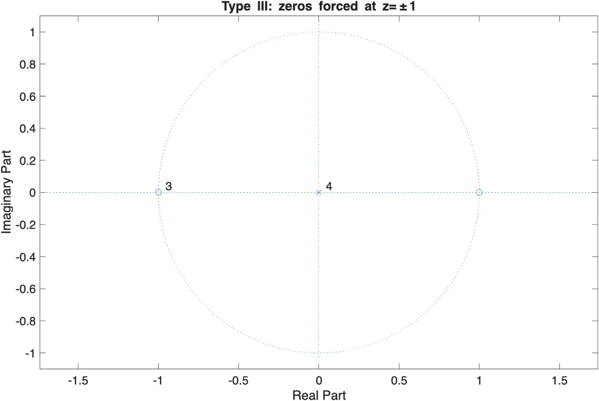
.png)
.png)