  ELEC6218 · Signal Processing
  Analog & Digital Filter Design

  Signal Processing · Lecture notes
  Prof. Çelik

ELEC6218 · Signal Processing

Lecture 6

Digital Filter Design

Digital filters fall into two main families. FIR filters are always stable and can have exactly linear phase, but they often need more coefficients. IIR filters can meet the same magnitude specification with a lower order, but their phase is usually nonlinear and their stability must be checked.

Quiz

Podcast

    InstructorProf. Abdulkadir Çelik (https://akadircelik.com)
    ModuleELEC6218
    TopicsFIR vs. IIR · exact linear phase · moving average · two-pole resonator · cascaded pole–zero design
  

    ▸ No feedback = guaranteed stability
    ▸ Symmetric taps = exact linear phase
    ▸ Feedback buys order at a price
    ▸ Cascade poles/zeros by hand
  

Learning outcomes

By the end of this lecture, you will be able to:

Distinguish FIR from IIR structurally, and explain why FIR is stable by construction while IIR requires a stability check.
Derive why symmetric FIR coefficients give exactly linear phase, and explain why no IIR or analog filter can match that guarantee.
Build and analyse the two simplest hand-designed filters — the FIR moving average and the IIR two-pole resonator — and compare their cost and risk.
Choose between FIR and IIR for a given application based on phase sensitivity, computational cost, and stability risk.

Lecture 6

Begin by comparing FIR and IIR structures, stability and phase. Then use a moving average, a one-pole low-pass and a two-pole resonator to see the trade-offs in concrete examples. The final section combines simple pole–zero sections into a multiband design.

iNotation used in this lecture

FIR

finite impulse response — feed-forward only, no feedback

IIR

infinite impulse response — feedback present, poles can be anywhere

\(M\)

FIR filter order — number of taps minus one

\(b_k,\;a_k\)

feed-forward and feedback coefficients (Lecture 4 notation)

\(r,\;\omega_0\)

pole radius and angle of a resonator/notch section

linear phase

phase exactly proportional to $\omega$; every frequency delayed equally

Purpose of this lecture. The hand-built examples develop intuition about FIR and IIR behaviour. Lecture 7 gives systematic FIR design methods, and Lecture 8 gives systematic IIR design methods.

6.1 Ideal digital filters, and the same four shapes again

Digital filters use the same ideal low-pass, high-pass, band-pass and band-stop shapes as analog filters. In discrete time, the responses repeat every $2\pi$ in $\omega$. The ideal brick-wall versions still cannot be implemented exactly because their inverse DTFT is an infinite, non-causal sinc:

Figure 6.1. The four ideal digital magnitude shapes, drawn over one period $-\pi\le\omega\le\pi$, plus a multiband example: several pass/stop regions built from the same brick-wall vocabulary, all equally unbuildable in ideal form.

Two realizable structures are available: FIR and IIR. This lecture compares their behaviour and trade-offs. Lecture 7 develops FIR design methods, while Lecture 8 develops IIR design from analog prototypes.

6.2 Two structures: FIR and IIR

Lecture 4's LCCDE (Eq. 4.12) splits into two structural cases depending on whether the feedback coefficients $a_k$ are present at all.

Recap from Lecture 4 · the LCCDE

Every filter in this lecture is one equation with two coefficient sets: $N$ feedback coefficients $a_k$ acting on past outputs, and $M+1$ feed-forward coefficients $b_k$ acting on present and past inputs.

$$\sum_{k=0}^{N}a_k\,y[n-k]=\sum_{k=0}^{M}b_k\,x[n-k] \qquad\Longleftrightarrow\qquad H(z)=\frac{\sum_{k=0}^{M}b_kz^{-k}}{\sum_{k=0}^{N}a_kz^{-k}}$$

The key distinction is feedback. With no feedback coefficients $a_k$, the filter is FIR. When past outputs are fed back, the denominator contains non-trivial poles and the filter is IIR.

FIR · no feedback

Set $a_0=1$ and $a_k=0$ for $k\ge1$. The denominator collapses to 1, so $H(z)$ is a polynomial in $z^{-1}$: only zeros, and $M$ poles stacked at $z=0$.

$$y[n]=\sum_{k=0}^{M}b_k\,x[n-k]$$

IIR · feedback present

At least one $a_k\neq0$ for $k\ge1$. The denominator survives, its roots are poles placed anywhere the designer likes, and stability becomes a condition to check.

$$y[n]=\sum_{k=0}^{M}b_k\,x[n-k]-\sum_{k=1}^{N}a_k\,y[n-k]$$

FIR
IIR

Stability

Guaranteed — poles only at $z=0$

Must be checked — poles can leave the unit circle

Phase

Can be made exactly linear (Section 6.3)

Generally non-linear, as Lecture 5 Problem 5.3 already showed for analog IIR

Order for a sharp cutoff

High — expensive

Low — efficient (this is exactly Lecture 5's Chebyshev/elliptic payoff)

Design method

Direct optimization on $\{b_k\}$ — minimize mean-squared error or the maximum error (minimax) (Lecture 7)

Transform an analog prototype (Lecture 8); direct optimization on $\{a_k,b_k\}$ is avoided — the cost surface is nonlinear, with local minima and no guarantee the poles stay inside the unit circle

Direct-form FIR block diagram: a chain of z-inverse delays on the input, each tapped by a coefficient b_k into a summation chain producing y[n] — **Figure 6.2.a.** The two structures drawn from the same equation. Left: the feed-forward half alone, a delay line tapped by $b_0\ldots b_M$ — Eq. (6.1) implemented literally, which is why $h[n]$ is the tap sequence. Right: the full LCCDE, the identical feed-forward half plus a second delay line on the output whose taps $-a_1\ldots-a_N$ return into the summation. That one added path is the entire structural difference between the families, and every entry in the table above traces back to it.

Direct-form I IIR block diagram: the same feed-forward delay chain and b_k taps on the left, plus a second delay chain on the output with taps minus a_k fed back into the summation — **Figure 6.2.a.** The two structures drawn from the same equation. Left: the feed-forward half alone, a delay line tapped by $b_0\ldots b_M$ — Eq. (6.1) implemented literally, which is why $h[n]$ is the tap sequence. Right: the full LCCDE, the identical feed-forward half plus a second delay line on the output whose taps $-a_1\ldots-a_N$ return into the summation. That one added path is the entire structural difference between the families, and every entry in the table above traces back to it.

6.2.1 FIR: finite impulse response

No feedback ($a_k=0$ for $k\ge1$); the output is a weighted sum of the $M+1$ most recent inputs only:

$$ y[n]=\sum_{k=0}^{M}b_k\,x[n-k], \qquad H(z)=\sum_{k=0}^{M}b_kz^{-k}, \qquad h[n]=\begin{cases}b_n,&0\le n\le M\\0,&\text{otherwise}\end{cases} $$

(6.1)

$h[n]$ literally is the coefficient sequence, finite by construction — there is no summation to infinity to justify.

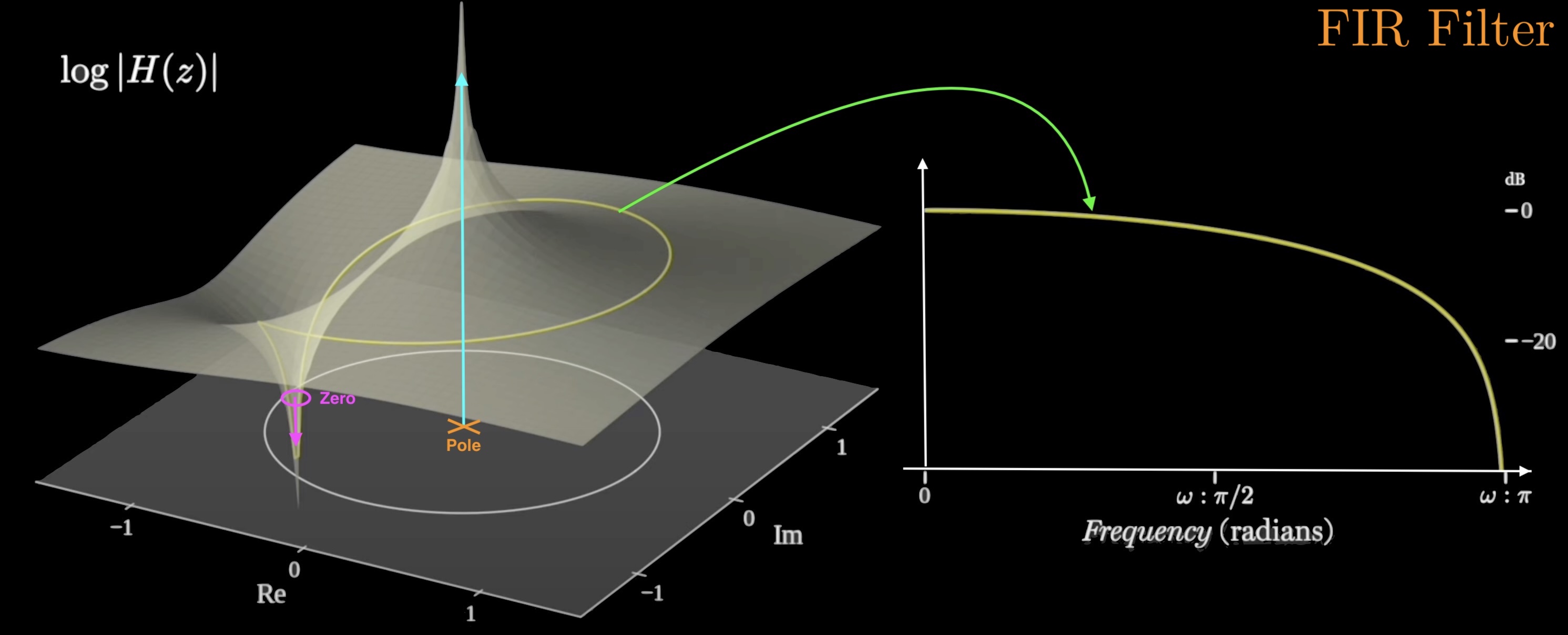
Three-dimensional log|H(z)| surface of an FIR filter, with its pole at the origin and one zero pulling the surface down, and the unit-circle slice drawn as the frequency response — **Figure 6.2.b.** An FIR filter seen as a surface. $\log|H(z)|$ is plotted over the whole $z$-plane: all $M$ poles sit stacked at the origin (the single spike), and the zeros pull the surface down towards $-\infty$. Reading the surface along the unit circle, exactly Eq. (4.16)'s geometric construction, gives the frequency response on the right. Because the only poles are at $z=0$, no choice of $b_k$ can ever move a pole outside the unit circle: FIR stability is structural, not a design constraint.

6.2.2 IIR: infinite impulse response

Feedback present: each output depends on past outputs as well as inputs, exactly Lecture 4's general LCCDE:

$$ y[n]=\sum_{k=0}^{M}b_k x[n-k]-\sum_{k=1}^{N}a_k y[n-k], \qquad H(z)=\frac{\sum_{k=0}^{M}b_kz^{-k}}{\sum_{k=0}^{N}a_kz^{-k}}\ \ (a_0=1) $$

(6.2)

For a stable IIR filter, partial fractions express the impulse response as a sum of decaying terms $A_k(d_k)^n u[n]$. These terms become very small but never become exactly zero, so the impulse response is mathematically infinite.

Three-dimensional log|H(z)| surface of the one-pole IIR filter y[n]=x[n]+0.9y[n-1], with the pole spike at z=0.9 and the resulting low-pass frequency response — **Figure 6.2.c.** The simplest IIR filter, $y[n]=x[n]+0.9\,y[n-1]$, as the same kind of surface. One feedback coefficient places one pole at $z=0.9$, just inside the unit circle; the surface rises towards $+\infty$ there, and the unit-circle slice nearest that spike is the low-frequency end, so the response is low-pass. Push the coefficient to $1.0$ and the spike lands on the circle: the same one added feedback path that buys the efficiency also puts stability into the designer's hands.

6.3 Why FIR can do what no analog filter can: exact linear phase

An FIR filter can achieve exact linear phase by using a symmetric coefficient sequence:

$$ b_k=b_{M-k}\ \ \text{(symmetric)} \quad\Longrightarrow\quad H(e^{j\omega})=|H(e^{j\omega})|\,e^{-j\omega M/2} $$

(6.3)

The phase is exactly $-\omega M/2$, so every passed frequency component is delayed by the same $M/2$ samples. The filter can therefore change the amplitude spectrum without changing the waveform shape, apart from a fixed delay. General causal IIR filters cannot provide this exact guarantee.

FIR pays with order

A sharp transition needs a long, symmetric coefficient sequence — large $M$, many multiplies per output sample.

IIR pays with phase

The same sharpness costs a handful of poles (Lecture 5's whole point) — but the phase that comes with them is not yours to choose.

This leads to the central trade-off. FIR filters are attractive when waveform shape must be preserved, for example in audio or biomedical signals. IIR filters are attractive when low computational cost is more important and some phase distortion is acceptable.

6.4 The simplest FIR low-pass: the moving average

Average the last $M$ samples and you already have a low-pass filter, with no design procedure at all:

$$ y[n]=\frac{1}{M}\sum_{k=0}^{M-1}x[n-k], \qquad H(z)=\frac{1}{M}\sum_{k=0}^{M-1}z^{-k}=\frac{1}{M}\cdot\frac{1-z^{-M}}{1-z^{-1}} $$

(6.4)

All $M$ coefficients equal $1/M$, so Eq. (6.3)'s symmetry condition is satisfied trivially — a moving average is linear-phase for free, delaying every frequency by exactly $(M-1)/2$ samples.

EXAMPLE 6.1 · The two-tap averager as an FIR low-pass

For $M=2$: $y[n]=0.5x[n]+0.5x[n-1]$. Find $H(z)$, its zero, and $|H(e^{j\omega})|$ at $\omega=0$ and $\omega=\pi$.

Step 1 · Transform. $h[n]=0.5\delta[n]+0.5\delta[n-1]$, so $H(z)=0.5+0.5z^{-1}=0.5(1+z^{-1})$, a single zero at $z=-1$ ($\omega=\pi$) and a pole at $z=0$ from the $z^{-1}$ term.

Step 2 · DC. $H(e^{j0})=0.5(1+1)=1$: a constant input passes through unattenuated — averaging cannot change a signal that is not changing.

Step 3 · Nyquist. $H(e^{j\pi})=0.5(1+e^{-j\pi})=0.5(1-1)=0$: the fastest-alternating sequence, $(-1)^n$, is annihilated completely — exactly what the zero at $z=-1$ guarantees, and exactly the behaviour Eq. (2.15)'s ladder predicted for the highest discrete-time frequency.

MATLAB corner for Example 6.1

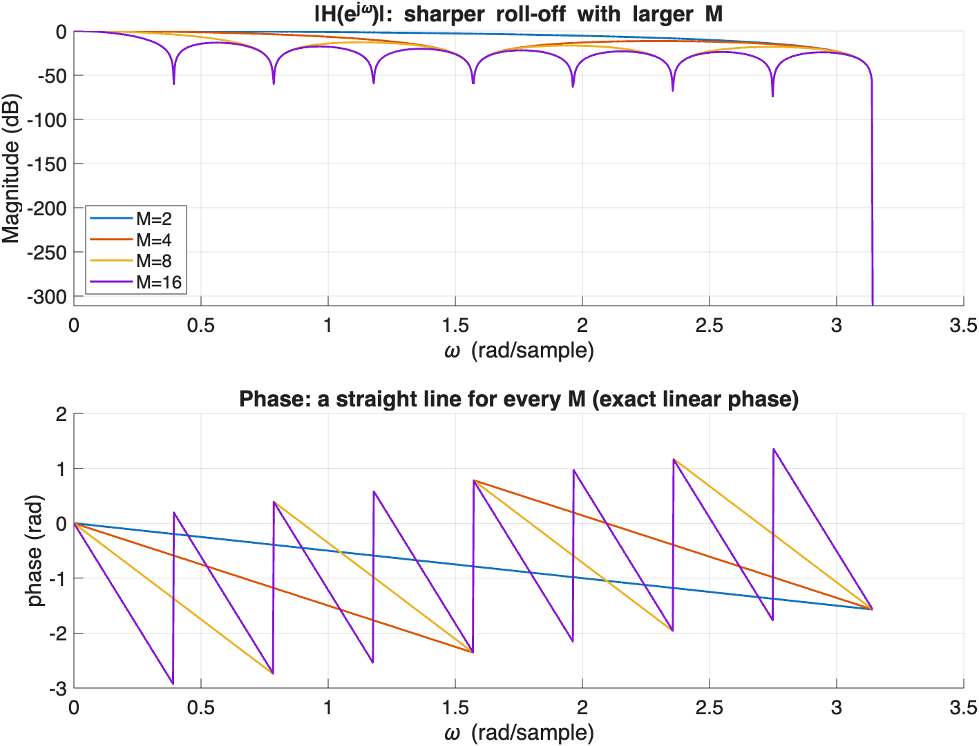
This script sweeps the averager length $M$ and confirms Eq. (6.3)'s promise directly: the phase stays perfectly linear no matter how the magnitude shape changes.

Goal: plot the magnitude and phase of a moving-average filter for several $M$, and verify the phase is exactly linear (a straight line) in every case.

moving_average_demo.m

MATLAB

%% moving_average_demo.m - FIR symmetry buys exact linear phase (Eq. 6.3)
Ms = [2 4 8 16];
w = linspace(0, pi, 1000);    % digital frequency (rad/sample)
figure('Color','w','Position',[100 100 700 500]);
 
colors = lines(numel(Ms));
subplot(2,1,1); hold on;
subplot(2,1,2); hold on;
 
for i = 1:numel(Ms)
    M = Ms(i);
    b = ones(1,M)/M;                 % moving-average taps
    H = freqz(b, 1, w);              % frequency response on [0,pi]
 
    subplot(2,1,1);
    plot(w, 20*log10(abs(H)+eps), 'Color', colors(i,:), 'LineWidth', 1.4);
 
    subplot(2,1,2);
    ph = unwrap(angle(H));
    plot(w, ph, 'Color', colors(i,:), 'LineWidth', 1.4);
end
 
% Magnitude plot
subplot(2,1,1);
grid on;
xlabel('\omega (rad/sample)');
ylabel('Magnitude (dB)');
title('|H(e^{j\omega})|: sharper roll-off with larger M');
legend(arrayfun(@(M)sprintf('M=%d',M), Ms, 'UniformOutput', false), 'Location','southwest');
 
% Phase plot
subplot(2,1,2);
grid on;
xlabel('\omega (rad/sample)');
ylabel('phase (rad)');
title('Phase: a straight line for every M (exact linear phase)');

Magnitude in dB and unwrapped phase of moving-average filters for M=2,4,8,16 — **Figure 6.4.a.** **Reading the moving-average results.** As the length $M$ increases, the main lobe becomes narrower and more zeros appear, so the filter separates low and high frequencies more sharply. This improvement requires more taps and therefore more computation and delay. Between the magnitude zeros, the phase is a straight line, which confirms linear phase. The apparent $\pi$-radian jumps occur where the real-valued frequency response changes sign at a zero; they do not represent a sudden change in physical delay.

6.4.1 The IIR twin: a one-pole low-pass, and a running audio-EQ example

Trade the moving average's feed-forward taps for one feedback term and the same low-pass job is done with a single pole instead of $M$ taps — the exponential smoother:

$$ y[n]=(1-a)x[n]+a\,y[n-1], \qquad H(z)=\frac{1-a}{1-az^{-1}}, \qquad 0<a<1 $$

(6.5)

The moving-average FIR and the one-pole IIR are two simple low-pass filters. Both have unity gain at DC, $H(1)=1$. The FIR response becomes sharper by adding taps. The IIR response is adjusted by moving one pole with the coefficient $a$, so it can be more efficient, but its phase is not linear. More complicated equalizers can be built by cascading several first- or second-order sections tuned to different frequency bands.

EXAMPLE 6.2 · Designing a one-pole low-pass shelf for an audio EQ

A bass-shelf stage in a 3-band digital audio EQ needs a one-pole low-pass (Eq. 6.5) with cutoff $f_c=200\,\text{Hz}$ at $f_s=48\,\text{kHz}$. Using the design rule $a=e^{-2\pi f_c/f_s}$, find $a$, write the difference equation, and compare its cost and stability margin to Example 6.1's moving average.

Step 1 · Solve for $a$. $a=e^{-2\pi(200)/48000}=e^{-0.02618}\approx0.9742$.

Step 2 · Difference equation. With $1-a\approx0.0258$: $y[n]=0.0258\,x[n]+0.9742\,y[n-1]$.

Step 3 · Cost. One pole, one multiply-add in feedback plus one in the feed-forward path: 2 multiplies, order 1, regardless of how low $f_c$ is set. An FIR moving average reaching a comparably low 200 Hz cutoff at 48 kHz would need roughly $M\approx f_s/f_c\approx240$ taps — the same order-vs-structure trade Example 6.3's resonator makes against a long FIR band-pass, now for a low-pass shelf.

Step 4 · Stability margin. The pole sits at $z=a\approx0.974$, safely inside the unit circle, but a fixed-point implementation that rounds $a$ up past 1 makes the filter's DC gain unbounded — unlike Example 6.1's moving average, whose only pole is fixed exactly at $z=0$ and cannot be dislodged by rounding.

MATLAB corner for Example 6.2

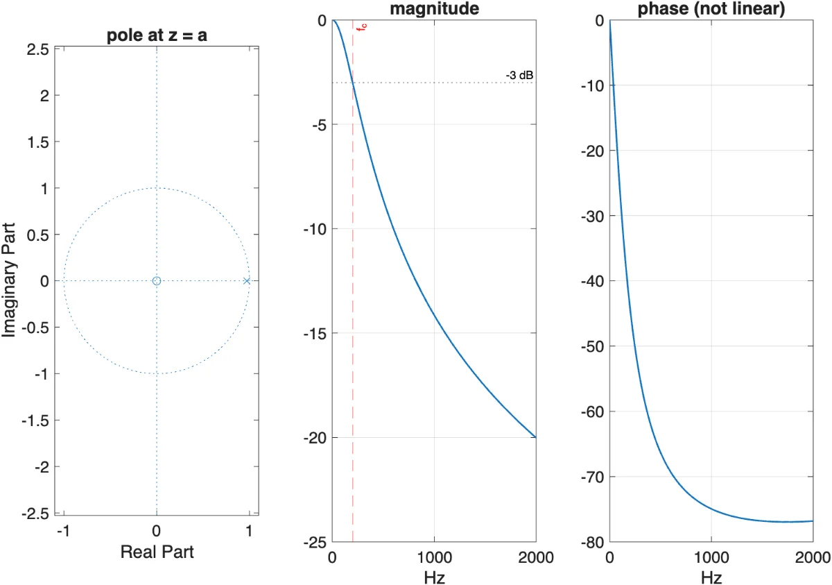
This script builds Example 6.2's bass-shelf filter, plots its pole, magnitude, and phase, and checks the design rule's $-3\,\text{dB}$ point numerically against the target $f_c$.

Goal: confirm $a=e^{-2\pi f_c/f_s}$ places the measured $-3\,\text{dB}$ point at (approximately) the target $f_c$, and show the phase curving smoothly rather than as a straight line.

onepole_iir_demo.m

MATLAB

%% onepole_iir_demo.m - Example 6.2's audio-EQ bass shelf (Eq. 6.5)
fc = 200; fs = 48000;
a = exp(-2*pi*fc/fs);                     % Eq. (6.5) design rule
b = [1-a]; den = [1 -a];
 
figure('Color','w');
subplot(1,3,1); zplane(b, den); title('pole at z = a');
[H,f] = freqz(b, den, 4096, fs);
subplot(1,3,2); plot(f, 20*log10(abs(H)), 'LineWidth',1.4); grid on;
xlim([0 2000]); xline(fc,'r--','f_c'); yline(-3,'k:','-3 dB');
title('magnitude'); xlabel('Hz');
subplot(1,3,3); plot(f, unwrap(angle(H))*180/pi, 'LineWidth',1.4); grid on;
xlim([0 2000]); title('phase (not linear)'); xlabel('Hz');
 
% verify the design rule numerically
[~, idx] = min(abs(20*log10(abs(H)) - (-3)));
fprintf('designed fc = %.1f Hz, measured -3dB point = %.1f Hz\n', fc, f(idx));

Figure 6.4.b — pole-zero, magnitude and phase produced by onepole_iir_demo.m — **Figure 6.4.b.** **Checking the one-pole IIR design.** The magnitude reaches $-3\,\text{dB}$ at 200 Hz, so the pole coefficient chosen from Eq. (6.5) meets the cutoff target. The response then rolls off smoothly because this is only a first-order filter. The phase curve is not a straight line: different frequency components experience different delays. Compare this with the moving-average FIR result in Figure 6.4.a, where the phase is linear between the zeros.

Figure 6.4.c. Following the pole–zero sweep. The filter has one pole at $z=a_1$ and one zero at $z=-b_1$. As $a_1$ increases towards 1, the pole moves closer to the unit circle near $\omega=0$. The low-frequency gain rises and the response becomes sharper. As $b_1$ increases towards 1, the zero moves towards $z=-1$, which corresponds to $\omega=\pi$, so the high-frequency gain falls towards zero. The animation separates the two effects: nearby poles increase the response, while nearby zeros reduce it.

6.5 The simplest IIR band-pass: the two-pole resonator

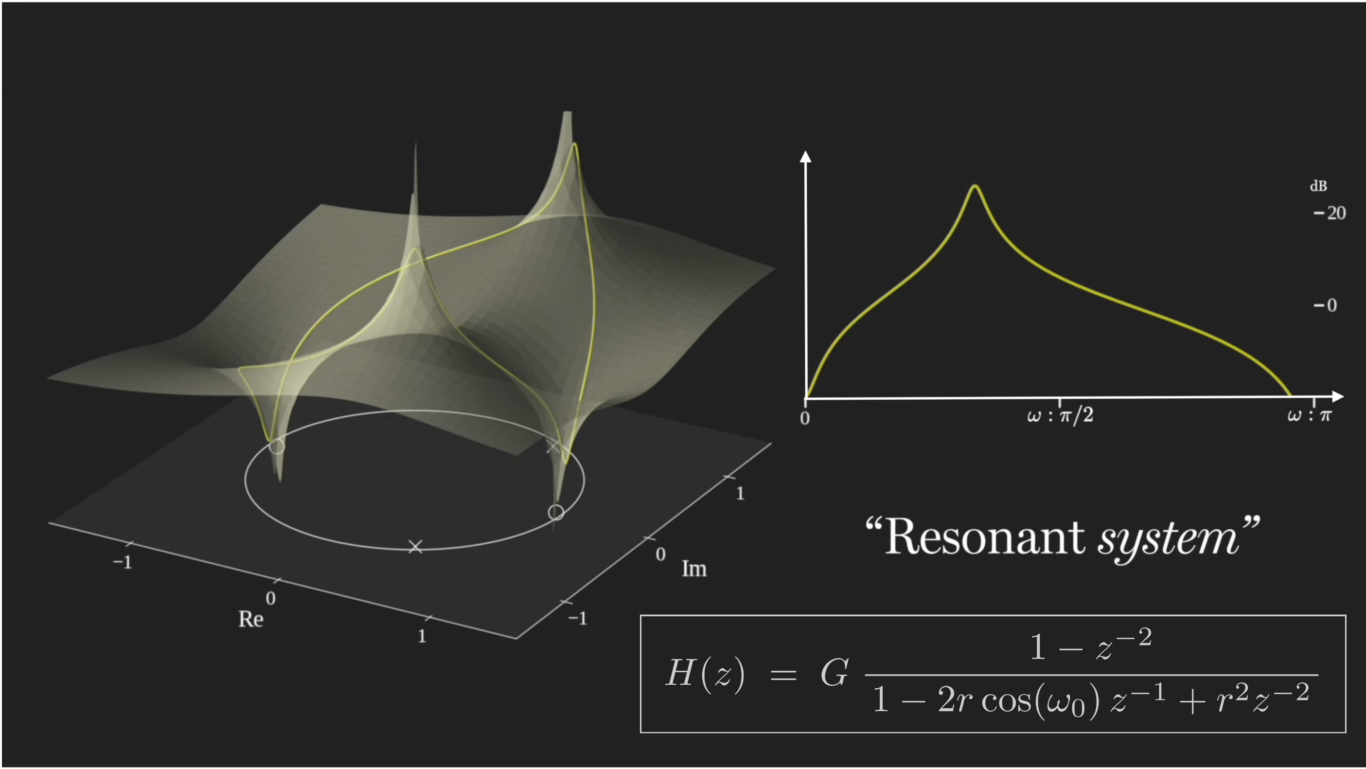
Place one conjugate pole pair close to the unit circle at angle $\omega_0$ and, exactly as Example 4.7's notch used zeros to create a null, a resonator uses poles to create a peak — the geometric method of Section 4.8 read in reverse:

$$ H(z)=\frac{1}{1-2r\cos\omega_0\,z^{-1}+r^2z^{-2}}, \qquad p_{1,2}=re^{\pm j\omega_0},\ \ r\lesssim1 $$

(6.6)

At $\omega=\omega_0$, the evaluation point on the unit circle is closest to the pole, so the magnitude reaches a peak. Moving the pole radius $r$ closer to 1 reduces this distance, producing a taller and narrower resonance. The pole angle sets the centre frequency, while the pole radius sets the bandwidth and ringing time.

Three-dimensional log|H(z)| surface of the resonant band-pass system, showing the conjugate pole pair spikes near the unit circle, the zeros at z=+-1, and the resulting peaked magnitude response — **Figure 6.5.a.** **How the resonator creates a band-pass response.** The zeros at $z=1$ and $z=-1$ force the response to zero at $\omega=0$ and $\omega=\pi$. The conjugate poles at $re^{\pm j\omega_0}$ create peaks near $\pm\omega_0$. Reading the surface around the unit circle therefore gives a response that starts at zero, rises to a resonance near $\omega_0$, and returns to zero at Nyquist. The pole angle chooses the centre frequency, while the radius $r$ controls the peak width and strength.

EXAMPLE 6.3 · Designing a two-pole resonator, and checking its cost

Design a resonator peaking at $f_0=1\,\text{kHz}$, $f_s=8\,\text{kHz}$, with $r=0.97$. Give the difference equation and compare its cost (multiplies, order) to an FIR filter that could produce a comparably narrow peak.

Step 1 · Angle. By Eq. (3.13), $\omega_0=2\pi f_0/f_s=2\pi(1000)/8000=\pi/4$.

Step 2 · Coefficients. $2r\cos\omega_0=2(0.97)(0.7071)\approx1.372$, $r^2\approx0.9409$, so $H(z)=1/(1-1.372z^{-1}+0.9409z^{-2})$ and

$$y[n]=x[n]+1.372\,y[n-1]-0.9409\,y[n-2].$$

Step 3 · Cost. Two multiplies, two delays, order 2 — regardless of how narrow $r=0.97$ makes the peak. An FIR filter reaching a comparably narrow passband would need dozens of taps (Figure 6.4.a's trend: sharper needs longer), i.e. tens of multiplies. This is Lecture 5's whole point about IIR efficiency, now demonstrated at the smallest possible scale: two poles do here what would need a much longer FIR filter.

Step 4 · The other side of the ledger. $|p|=0.97<1$ so it is stable, but only just: rounding the coefficients in a fixed-point implementation could push a pole outside the unit circle. No such risk exists for the FIR alternative, whose only pole sits at $z=0$ regardless of coefficient rounding — the stability-must-be-checked row of Section 6.2's table, concretely.

MATLAB corner for Example 6.3

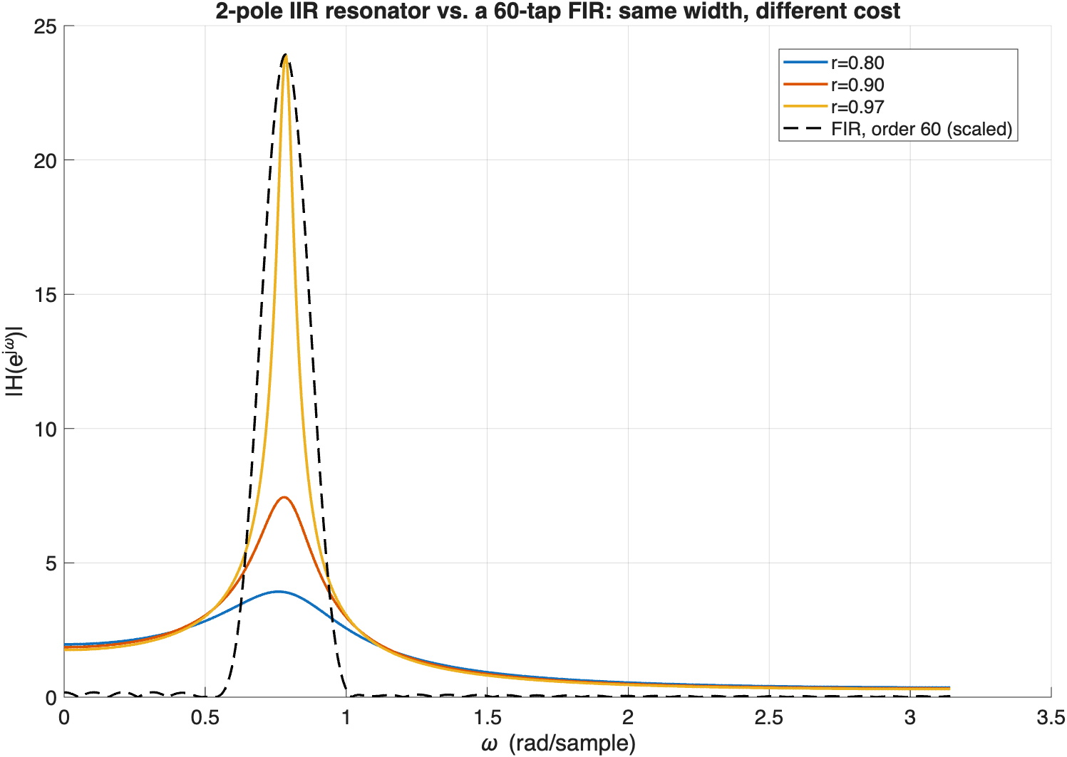
This script builds Example 6.3's resonator, sweeps $r$ to show the peak sharpen exactly as Section 4.8's geometric argument predicts, and overlays a long FIR band-pass of comparable width to make the order comparison from Step 3 visible.

Goal: confirm the resonator's peak sharpens as $r\to1$, and compare its 2-pole cost to an FIR filter needed for a similarly narrow passband.

resonator_vs_fir_fixed.m

MATLAB

% resonator_vs_fir_fixed.m - two IIR poles vs. many FIR taps (Eq. 6.6, Sec. 4.8)
w0 = pi/4;
w = linspace(0, pi, 2000);
figure('Color','w');
hold on;
 
rs = [0.8 0.9 0.97];
colors = lines(numel(rs));
for i = 1:numel(rs)
    r = rs(i);
    b = 1;
    a = [1, -2*r*cos(w0), r^2];        % Eq. (6.6)
    Hi = abs(freqz(b, a, w));          % frequency response magnitude
    plot(w, Hi, 'Color', colors(i,:), 'LineWidth', 1.8);
end
 
% FIR bandpass design (fallback if fir1 not available)
Nfir = 60;                                % FIR order
Wp = [w0-0.05, w0+0.05];                 % passband in rad/sample
Wn = Wp/pi;                              % normalized to [0,1] for fir1
 
if exist('fir1','file')
    bfir = fir1(Nfir, Wn, 'bandpass');
else
    % simple windowed-sinc bandpass fallback
    M = Nfir;
    n = 0:M;
    fc1 = (Wp(1))/pi; fc2 = (Wp(2))/pi;  % normalized
    hbp = sinc(2*fc2*(n-M/2)).* (2*fc2) - sinc(2*fc1*(n-M/2)).*(2*fc1);
    wwin = 0.5*(1 - cos(2*pi*n/(M)));    % Hann (periodic) window
    bfir = hbp .* wwin;
end
 
Hfir = abs(freqz(bfir, 1, w));
% scale FIR to match peak of the narrowest IIR for fair visual comparison
peakIIR = max(abs(freqz(1, [1 -2*rs(end)*cos(w0) rs(end)^2], w)));
scale = peakIIR / max(Hfir);
plot(w, scale*Hfir, 'k--', 'LineWidth', 1.6);
 
grid on;
legend_entries = [arrayfun(@(r)sprintf('r=%.2f',r), rs, 'UniformOutput', false), ...
                  {sprintf('FIR, order %d (scaled)', Nfir)}];
legend(legend_entries, 'Location', 'northwest');
xlabel('\omega (rad/sample)'); ylabel('|H(e^{j\omega})|');
title('2-pole IIR resonator vs. a 60-tap FIR: same width, different cost');

Two-pole IIR resonator magnitude for r=0.80, 0.90, 0.97 overlaid with a scaled 60-tap FIR band-pass — **Figure 6.5.b.** **IIR resonator and FIR filter compared.** The pole angle fixes the centre frequency of the IIR resonance. Moving the radius $r$ closer to 1 brings the poles nearer the unit circle, making the peak taller and narrower while leaving its centre in the same place. Only two poles are needed. The FIR design needs about 60 taps to obtain a similarly narrow band, which illustrates the efficiency advantage of IIR filters. The trade-off is that the IIR response has nonlinear phase and becomes more sensitive as its poles approach the stability boundary.

6.6 Parametric design: cascading pole–zero building blocks

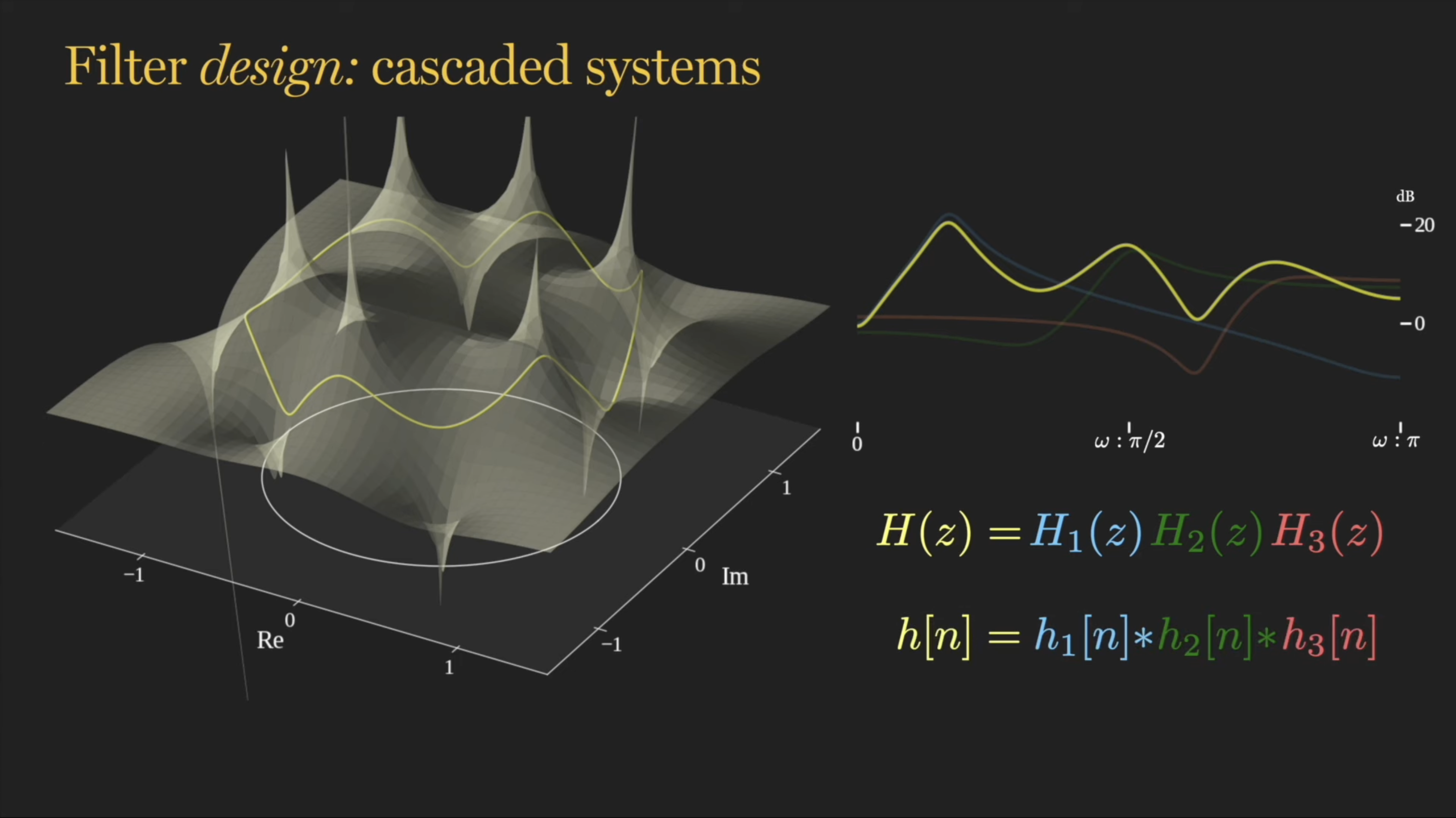
A resonator, notch or shelf can be designed as a simple pole–zero section. Several sections can then be connected in series to build a more complicated response. Cascading multiplies their transfer functions, so a three-band equalizer can be written as

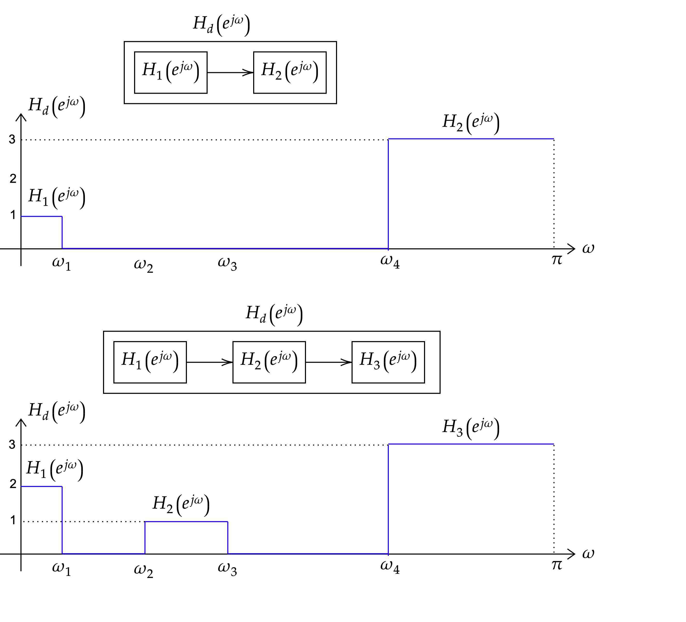
$$ H_{\text{eq}}(z)=H_1(z)\,H_2(z)\,H_3(z), \qquad \text{each } H_i \text{ a low-order resonator/notch section.} $$

(6.7)

Two piecewise-constant desired magnitude specifications, each drawn beneath a block diagram showing it realised as a cascade of two and of three sub-filters — **Figure 6.6.a.** Why cascading is the natural way to meet a multi-band specification. A desired response $H_d(e^{j\omega})$ made of separated bands at different gains is not one filter to be designed at once; each band is handed to its own section, and the sections are placed in series. Two bands need two sections (top), three need three (bottom), and each section is designed against the single, simple feature it owns.

Each section controls one local feature, such as a peak, notch or shelf. Because transfer functions multiply, their magnitude responses add when plotted in decibels. This approach works well for a small number of separated features; precise band-edge specifications are better handled by the systematic methods in Lectures 7 and 8.

Building intuition: watch the poles and zeros move

Use a pole–zero explorer to connect geometry with the response. Moving a pole towards the unit circle raises and narrows the nearby peak. Moving a zero onto the unit circle creates an exact null at its angle. The figures in this lecture are fixed examples of the same continuous relationship.

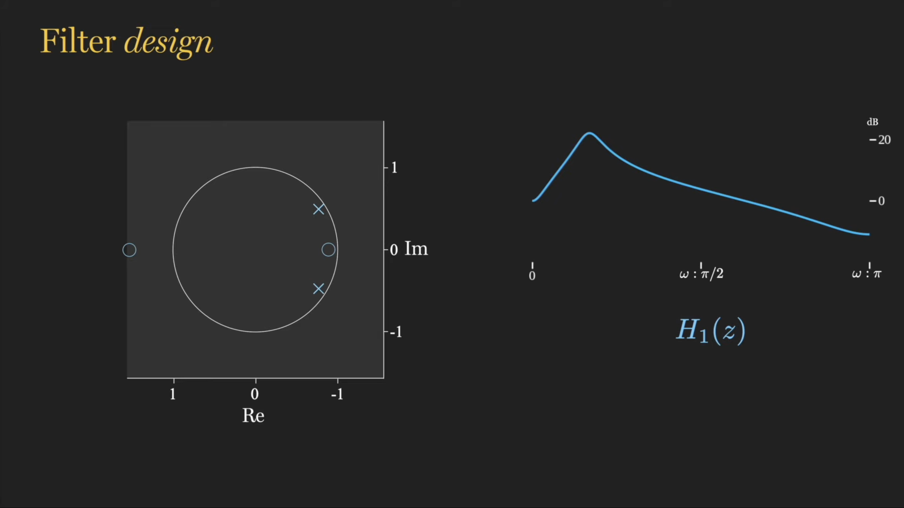
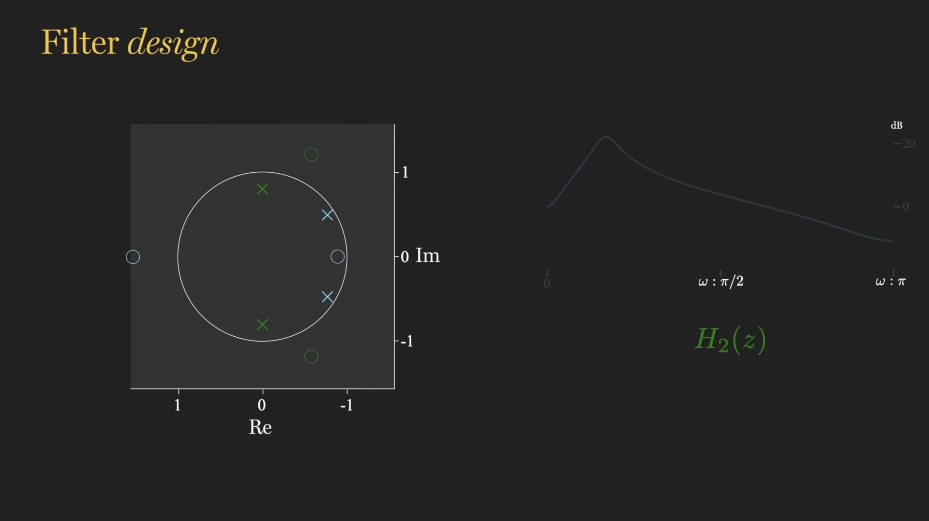
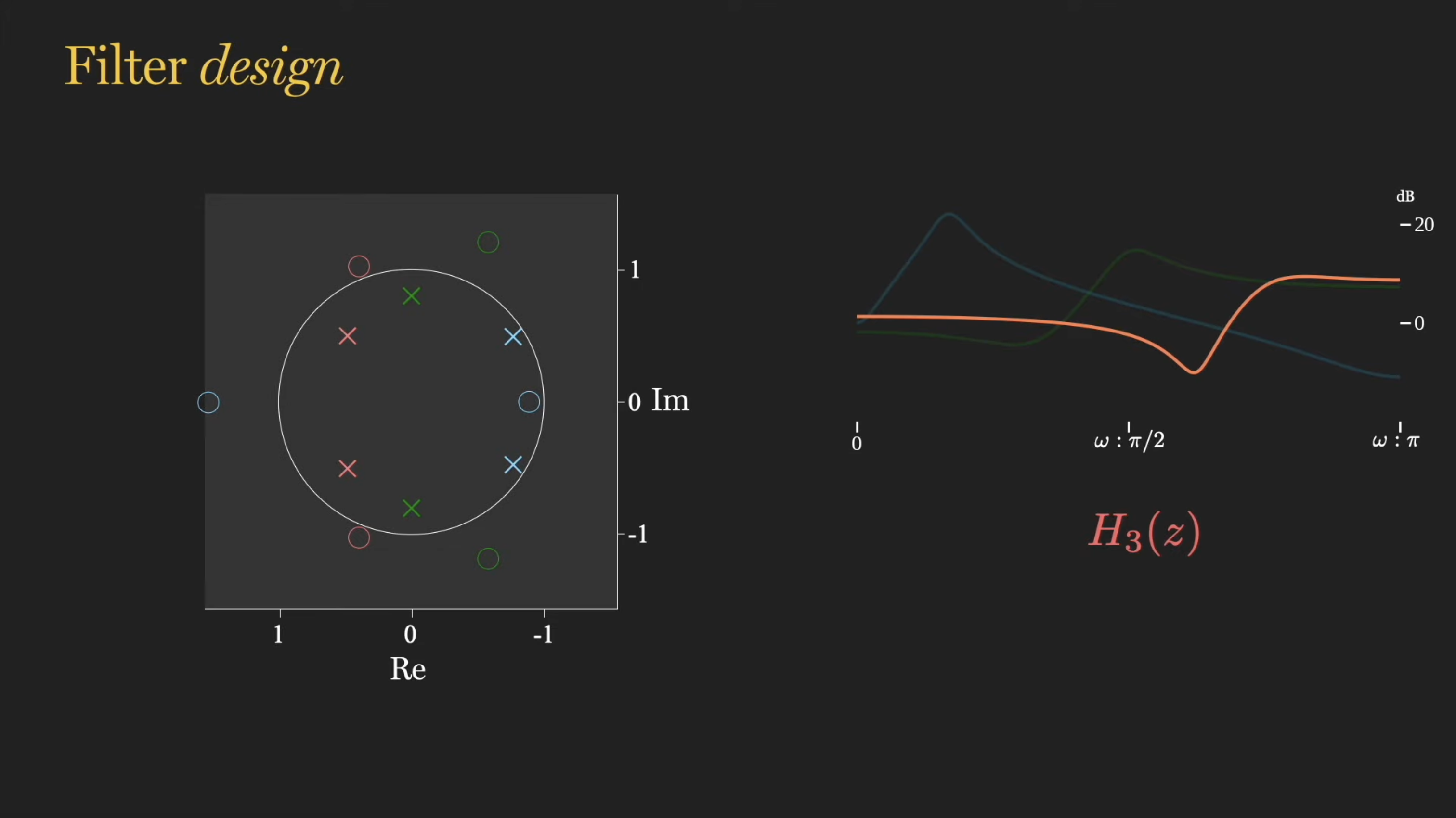
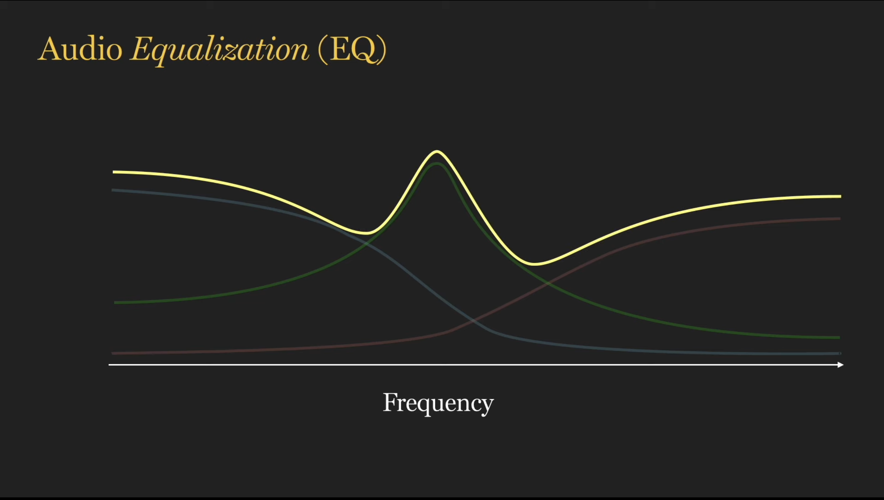
Pole-zero plot and magnitude response of H1(z) alone, a single conjugate pole pair giving one low-frequency peak — **Figure 6.6.b.** **Building the cascade one section at a time.** The first three panels add the blue, green and red pole–zero sections separately. Each section creates a local peak or dip near its own pole–zero pair without moving the features already designed. The final panel shows their product in yellow. Because $H(z)=H_1(z)H_2(z)H_3(z)$, the magnitudes multiply; on a dB scale, the three section responses add. This is why a complicated response can be designed as several simpler sections.

Pole-zero plot with H2(z) added in green, its second pole pair adding a mid-band feature to H1 — **Figure 6.6.b.** **Building the cascade one section at a time.** The first three panels add the blue, green and red pole–zero sections separately. Each section creates a local peak or dip near its own pole–zero pair without moving the features already designed. The final panel shows their product in yellow. Because $H(z)=H_1(z)H_2(z)H_3(z)$, the magnitudes multiply; on a dB scale, the three section responses add. This is why a complicated response can be designed as several simpler sections.

Three such sections, one tuned per band, and cascaded per Eq. (6.7), build a simple graphic equalizer:

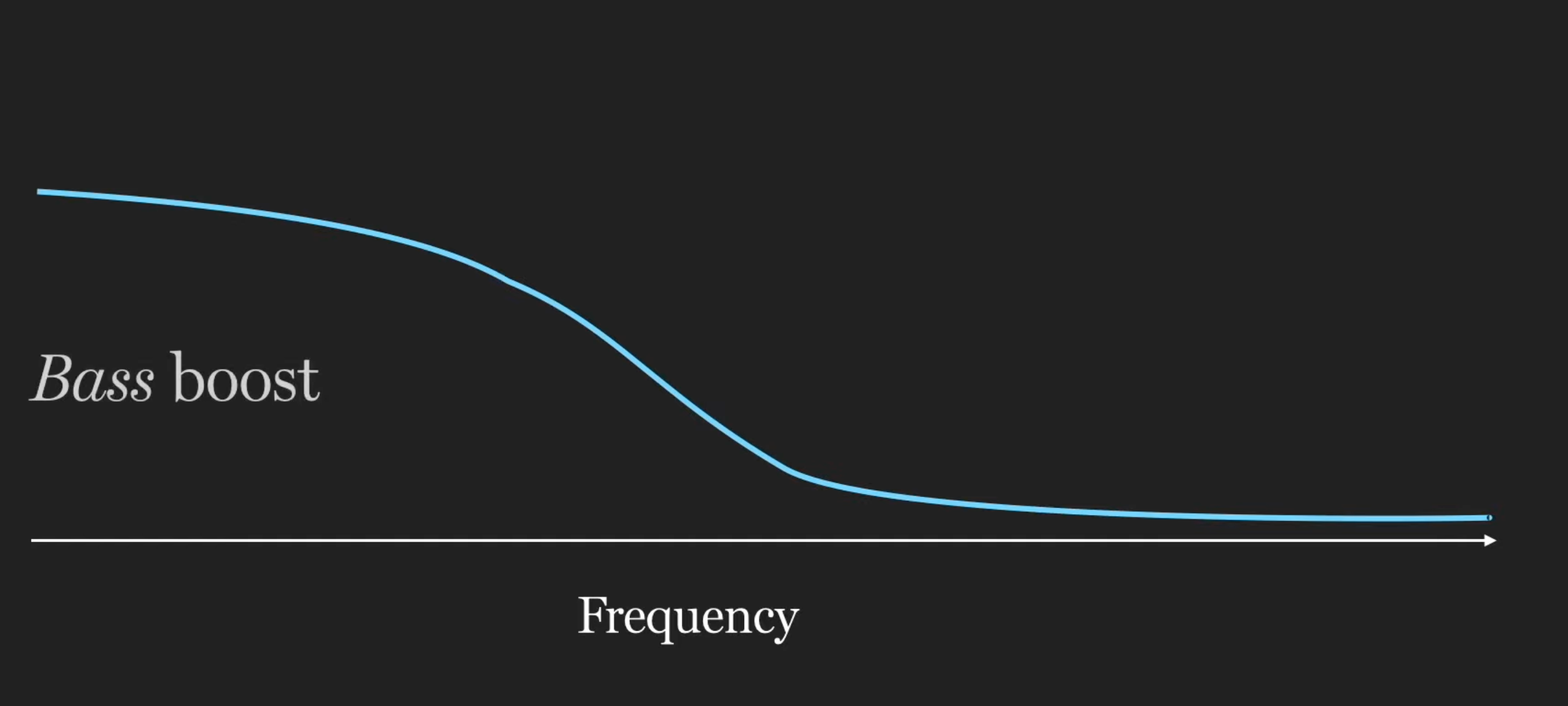
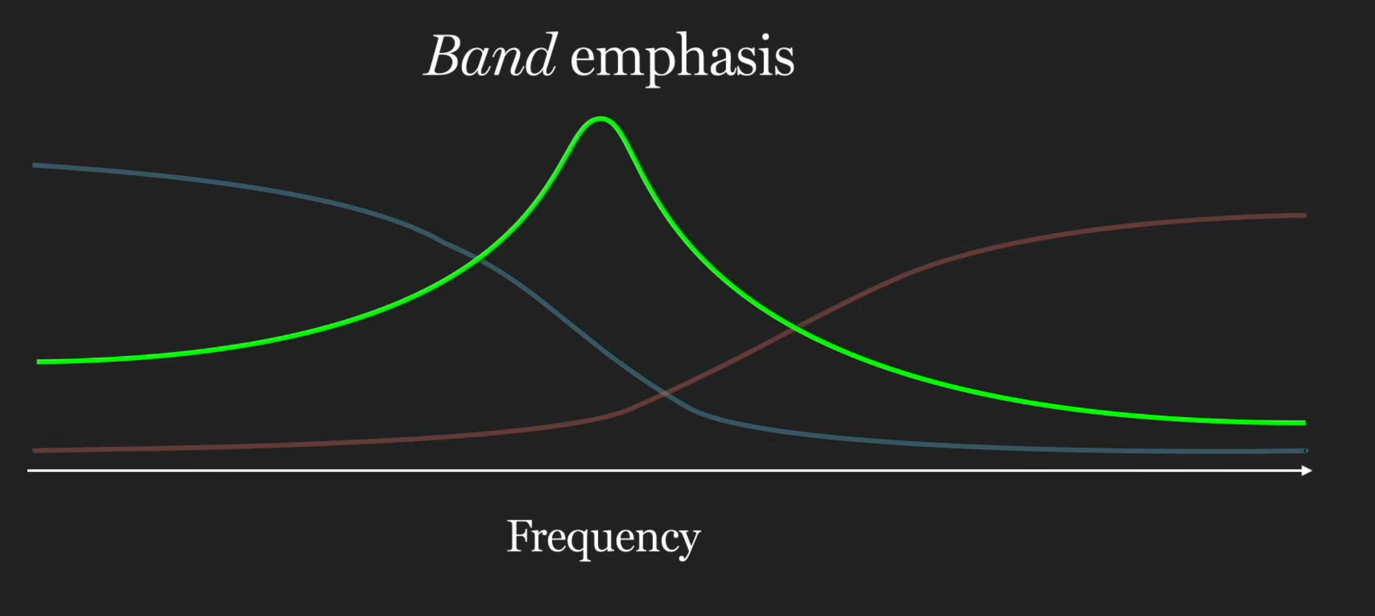
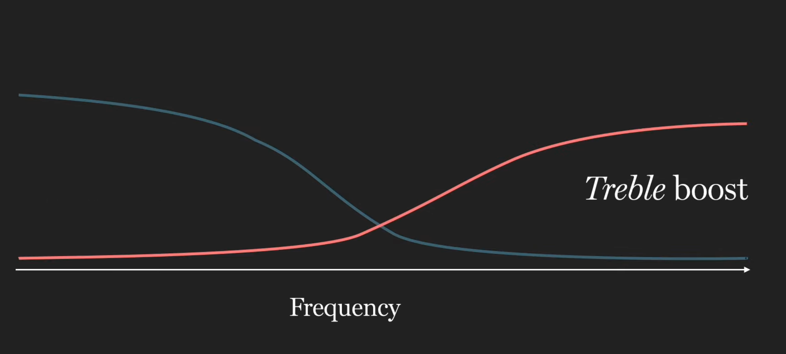
H1(z): bass boost, a low-frequency shelf — **Figure 6.6.c.** **Interpreting the three-band equalizer.** The top row shows the sections separately: $H_1$ controls the bass, $H_2$ adds a mid-band peak, and $H_3$ controls the treble. The yellow curve at the bottom is the cascade. Each local feature remains centred at the frequency chosen for its section, while overlapping gains combine. Since gains add in dB, raising one section lifts the combined curve mainly in that section's frequency range.

H2(z): band emphasis, a mid-frequency peak — **Figure 6.6.c.** **Interpreting the three-band equalizer.** The top row shows the sections separately: $H_1$ controls the bass, $H_2$ adds a mid-band peak, and $H_3$ controls the treble. The yellow curve at the bottom is the cascade. Each local feature remains centred at the frequency chosen for its section, while overlapping gains combine. Since gains add in dB, raising one section lifts the combined curve mainly in that section's frequency range.

?Problems with solutions

Work each one before reading the solution.

PROBLEM 6.1

A three-tap FIR filter has $b_0=b_2=0.25$, $b_1=0.5$. Verify it satisfies Eq. (6.3)'s symmetry condition, and find its exact phase delay in samples.

Solution. With $M=2$, Eq. (6.3)'s condition is $b_k=b_{2-k}$: $b_0=b_2=0.25\ \checkmark$ and $b_1=b_1$ trivially. So the phase is exactly $-\omega M/2=-\omega$, a delay of exactly $\boxed{1\text{ sample.}}$

Note this is a different (and smoother) three-tap averager than Example 6.1's two-tap one — the weights $0.25,0.5,0.25$ taper toward the edges, which by the window intuition of Lecture 5 (Section 5.2, Step 4) gives lower sidelobes than the equal-weight moving average, at the cost of a slightly wider main lobe.

PROBLEM 6.2

A resonator (Eq. 6.6) with $r=0.995$ needs 16-bit fixed-point coefficients. Explain, without computing anything, why this design is riskier to implement than Example 6.1's moving average at the same word length.

Solution. The resonator's stability depends entirely on its pole radius satisfying $|p|<1$ (Lecture 4, Eq. 4.8); with $r=0.995$ the pole sits only $0.005$ inside the unit circle, so a small rounding error in the quantized coefficients $2r\cos\omega_0$ or $r^2$ can push the effective pole radius past 1 and make the filter unstable — exactly the risk flagged in Section 6.2's table and Example 6.3 Step 4.

The moving average has no such exposure: its only pole is fixed exactly at $z=0$ by construction (Eq. 6.1's structure), so no amount of coefficient rounding can move it outside the unit circle. This is the FIR-guaranteed-stability row of the comparison table made concrete: guaranteed by structure, not by a numerical margin that can be eroded by quantization.

PROBLEM 6.3

A biomedical ECG system must remove 50 Hz mains hum without distorting the QRS complex's waveform shape. Which family, FIR or IIR, is the safer default, and why? (Compare to Example 4.7's IIR notch.)

Solution. FIR is the safer default whenever waveform shape itself is the clinically meaningful signal, which is exactly the ECG case: a symmetric linear-phase FIR notch (Eq. 6.3) delays the QRS complex's every frequency component by the same amount, so the complex re-emerges time-shifted but otherwise undistorted — Section 6.3's point made in an application.

Example 4.7's IIR notch removes the same 50 Hz tone with far fewer coefficients (a real practical advantage when compute is constrained), but its non-linear phase near the notch means different frequency components of the QRS complex are delayed by slightly different amounts, subtly distorting its shape — usually acceptable for a communications signal, less so when a clinician is reading morphology off the waveform.

PROBLEM 6.4*

Three resonator sections (Eq. 6.6) are cascaded per Eq. (6.7), each with a different $\omega_0$ but the same $r$. Explain why the combined magnitude in dB is the sum of the three individual magnitude curves in dB, and what this implies for placing the three peaks close together. (* optional)

Solution. Cascading multiplies the transfer functions, $H=H_1H_2H_3$ (Eq. 6.7), so $|H|=|H_1||H_2||H_3|$, and taking $20\log_{10}$ of a product turns it into a sum: $20\log_{10}|H|=\sum_i20\log_{10}|H_i|$ — logarithms convert the multiplicative combination of cascaded stages into the additive one a dB plot displays directly.

If the three peaks are placed close together in frequency, each resonator's response has not yet decayed back to $0\,\text{dB}$ at its neighbours' centre frequencies, so the sum raises the floor between the peaks — the equalizer bands interact rather than staying independent. Keeping the peaks well separated relative to each section's $3\,\text{dB}$ width (itself set by $r$, Example 6.2) is what keeps the three bands acting independently, exactly the same separation logic Lecture 5's frequency transformations relied on for clean band edges.

Summary and key formulas

The reference sheet: the two structures, the trade between them, and the two simplest hand-built filters of each type.

FIR · Eq. (6.1)

$$H(z)=\sum_{k=0}^{M}b_kz^{-k}$$

IIR · Eq. (6.2)

$$H(z)=\frac{\sum_k b_kz^{-k}}{\sum_k a_kz^{-k}}$$

Exact linear phase · Eq. (6.3)

$$b_k=b_{M-k}\Rightarrow \angle H=-\omega M/2$$

Moving average · Eq. (6.4)

$$y[n]=\tfrac{1}{M}\textstyle\sum_{k=0}^{M-1}x[n-k]$$

One-pole IIR · Eq. (6.5)

$$H(z)=\tfrac{1-a}{1-az^{-1}}$$

Resonator · Eq. (6.6)

$$H(z)=\tfrac{1}{1-2r\cos\omega_0 z^{-1}+r^2z^{-2}}$$

Cascade · Eq. (6.7)

$$H_{\text{eq}}=H_1H_2H_3,\ \ \text{dB adds}$$

The same four ideal shapes as analog filters (Lecture 5) return in discrete time, periodic in $\omega$, and are equally unbuildable in their ideal form.
FIR has no feedback, hence guaranteed stability (only a pole at $z=0$) and, with symmetric coefficients, exactly linear phase — a guarantee no analog or IIR prototype in this module can match.
IIR has feedback, hence a much lower order for a given sharpness (inherited directly from Lecture 5's Chebyshev/elliptic advantage), at the cost of non-linear phase and a stability condition that must be checked, not assumed.
A moving average is the simplest FIR low-pass: all-equal taps, linear phase for free, a zero at $\omega=\pi$ that nulls the fastest-alternating sequence exactly.
A one-pole IIR low-pass (Eq. 6.5) does the same job with a single feedback term instead of $M$ taps, at the cost of non-linear phase — the smallest possible instance of Section 6.3's trade.
A two-pole resonator is the simplest IIR band-pass: one conjugate pole pair near the circle, peak sharpness set by how close $r$ is to 1, at a stability cost that grows as $r\to1$.
Cascading low-order pole/zero sections (Eq. 6.7) is hand-built parametric design — effective for a few separated features, superseded by systematic methods once the specification is a single precisely-shaped band edge.
Next: Lecture 7 builds FIR filters systematically (windowing, Parks-McClellan); Lecture 8 builds IIR filters systematically by transforming Lecture 5's analog prototypes with the bilinear transform.

Digital Filter Design

Contents

6.1 Ideal digital filters, and the same four shapes again

6.2 Two structures: FIR and IIR

6.2.1 FIR: finite impulse response

6.2.2 IIR: infinite impulse response

6.3 Why FIR can do what no analog filter can: exact linear phase

6.4 The simplest FIR low-pass: the moving average

6.4.1 The IIR twin: a one-pole low-pass, and a running audio-EQ example

6.5 The simplest IIR band-pass: the two-pole resonator

6.6 Parametric design: cascading pole–zero building blocks

?Problems with solutions

Summary and key formulas