Introduction to
Signals & Systems
A signal carries information. A system receives a signal and produces a new one. In this lecture, you will learn how to describe signals and systems, decide whether a system is linear and time-invariant, and use convolution to calculate its output. These ideas are the foundation for the transforms and filter designs used later in the module.
Contents
Start with the main ideas, then use the worked examples, MATLAB activities and practice problems to check your understanding.
1.1 Signals, systems, and the three classic problems
A signal is a quantity that carries information. For example, it may represent a microphone voltage, a temperature measurement or a sequence of image pixels. A continuous-time (CT) signal is written as \(x(t)\), where \(t\) can take any real value. A discrete-time (DT) signal is written as \(x[n]\), where \(n\) is an integer sample index. A system is anything that changes an input signal into an output signal. It may be a physical circuit, a communication channel, a software algorithm or a natural process:
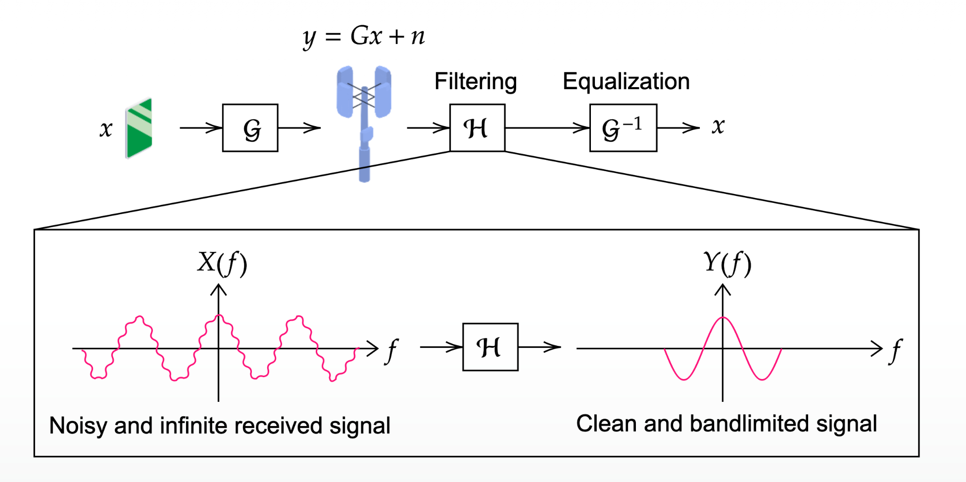
Most signal-processing questions belong to one of three groups:
- System identification. Given \(x\) and \(y\), determine \(\mathcal{H}\).
- Filtering. Given \(x\) and \(\mathcal{H}\), compute \(y\).
- Equalization (the inverse problem). Given \(y\) and \(\mathcal{H}\), estimate \(x\).
The first example is a wireless link. The transmitter sends \(x\), the channel \(\mathcal{G}\) changes it, and noise \(n\) is added. The receiver therefore observes \(y = \mathcal{G}x + n\).
The second example shows both the value and the limits of digital processing. Hubble's faulty optics acted as an unwanted system \(\mathcal{H}\), so the recorded image was a blurred version of the true scene plus noise: \(y = \mathcal{H}\{x\} + n\).
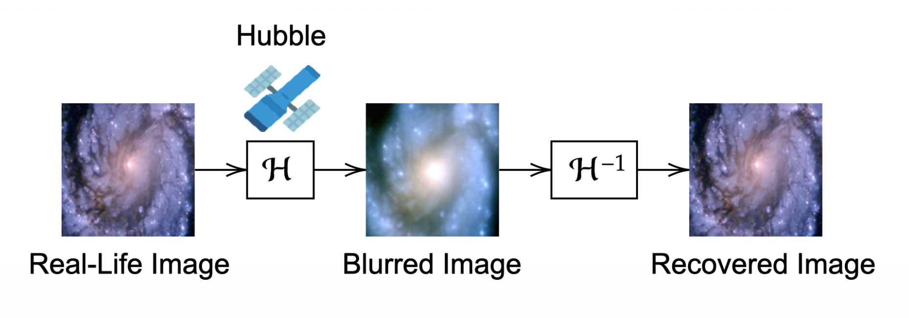
NASA launched Hubble in 1990. Its first images showed that stars appeared with a halo instead of as sharp points. The edge of the 2.4 m primary mirror was about 2.2 µm too flat because the equipment used to test the mirror had been assembled incorrectly. Light reflected from different parts of the mirror therefore came to focus at different positions. This effect is called spherical aberration.
Before the telescope could be repaired, engineers used signal processing to improve the images. They first estimated the point spread function from images of stars. This identified the unwanted optical system \(\mathcal{H}\). They then applied deconvolution, which acts like an approximate inverse \(\mathcal{H}^{-1}\). The method helped with bright, compact objects, but it also amplified noise and could not recover light that had fallen outside the detector.
A servicing mission provided the permanent solution in 1993. Astronauts installed corrective optics and a new camera designed to compensate for the mirror error. Instead of correcting the image after the distortion had occurred, the new hardware corrected the optical system itself.
Engineering lesson. Equalization can reduce known distortion, but it cannot recreate information that was never measured. Whenever possible, improve the system that produces the signal. If that is not possible, identify the system carefully and accept that its inverse will be approximate.
System identification, filtering and equalization appear in audio, communications, radar, sonar, biomedical engineering and computer vision. The mathematics is similar; only the physical meaning of the signals and systems changes.
1.1.1 Analog electronics, and why we still need it
Analog systems use physical components such as resistors, capacitors, inductors, diodes, transistors and operational amplifiers. They remain important because they can work over a wide frequency range with low delay and low power. Every digital processor also needs analog circuits at its input and output. The circuit below is a simple band-pass filter: a series resistor \(R\) feeds a parallel inductor-capacitor branch, and \(U_{\text{out}}\) is measured across that branch.
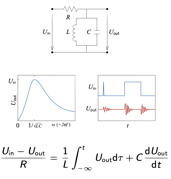
We obtain the circuit equation by applying Kirchhoff's current law at the node after \(R\). Ohm's law gives the resistor current as \((U_{\text{in}}-U_{\text{out}})/R\). This current divides between the inductor and capacitor. Their currents are \(i_L=\frac{1}{L}\int_{-\infty}^{t}U_{\text{out}}(\tau)\,d\tau\) and \(i_C=C\,dU_{\text{out}}/dt\). Therefore:
Equation (1.1) contains both an integral and a derivative of \(U_{\text{out}}\). To put it into a standard form, differentiate every term once. The derivative of the integral is simply \(U_{\text{out}}\):
Next, move all output terms to the left and keep the input term on the right. Divide by \(C\) so that the coefficient of the highest derivative is 1:
The result is a second-order linear constant-coefficient differential equation (LCCDE). Its undamped resonant frequency is \(\Omega_0=\sqrt{1/(LC)}\), which agrees with the frequency of the peak in the graph:
In an LCCDE, the input, output and their derivatives appear only to the first power, and their coefficients do not change with time:
This form tells us that the system is linear and time-invariant. Linearity comes from using only first powers; constant coefficients mean that the rule does not change with time. A transform can then replace differentiation with multiplication, turning the differential equation into an algebraic equation. The coefficient sets \(\{a_k\}\) and \(\{b_m\}\) determine the system's poles and zeros. In discrete time, difference equations play the same role, with delays replacing derivatives.
At \(\Omega_0\), the inductor and capacitor currents are equal in size and opposite in direction. For ideal components, they cancel, so the parallel branch has a very high impedance. Very little voltage is then lost across \(R\), and \(U_{\text{out}}\approx U_{\text{in}}\). Away from resonance, the branch impedance becomes smaller and more voltage appears across \(R\). The output therefore falls on both sides of \(\Omega_0\), producing a band-pass response.
The bottom-right plot shows the same filter in the time domain. A narrow test pulse approximates an impulse, so the resulting decaying oscillation is the impulse response \(h(t)\). Its oscillation frequency is close to \(\Omega_0\). A rectangular input has two sharp edges, and each edge starts a new period of ringing. Between the edges the input is constant, so little energy is present near the resonant frequency. The frequency and time plots describe the same behaviour: a taller, narrower resonance usually produces ringing that lasts longer. A filter cannot be extremely selective in frequency and settle instantly in time.
This simple RLC circuit introduces ideas that return throughout the module. Lecture 5 uses several poles to shape a complete analog passband. Lecture 2 shows that the frequency response is the Fourier transform of the impulse response. In Lecture 6, a digital two-pole resonator replaces the component values \(R\), \(L\) and \(C\) with a pole radius and angle in the \(z\)-plane. Lecture 8 then converts analog prototypes into digital IIR filters. The same link between pole position, frequency selectivity and ringing appears in every case.
1.1.2 Why go digital at all
Analog filters remain valuable. They need no sampling clock or software and can operate at very high frequencies. Their limitation is flexibility. Component values vary with tolerance, temperature and age, and these errors accumulate in a high-order circuit. Once the circuit is built, changing its cutoff usually means changing hardware. A digital filter stores its design as coefficients, so it can be reproduced accurately, retuned, or adapted while it is running. Digital processing also supports operations such as exact linear-phase FIR filtering and data-dependent decisions that a passive analog network cannot provide.
In a digital filter, the design is stored as numerical coefficients. The same coefficients can be copied exactly to another device and changed without replacing hardware. A high-order filter requires more calculations, but not a large network of physical components. Software can also adapt the filter, process signals at several sample rates, or operate on a complete stored recording.
However, microphones, antennas and sensors produce analog voltages rather than numbers. A practical digital system therefore has three stages: convert the analog input into samples, process the samples, and convert the result back into an analog signal when required. Figure 1.1.e shows this complete path.
Digital processing does not remove the need for analog electronics. Instead, the two technologies share the work:
Analog circuits are not limited by a sampling rate and introduce no data-conversion delay. Passive networks may need no power. They are also essential around every converter: an anti-alias filter is needed before an ADC, and a reconstruction filter is needed after a DAC.
Digital filters are reproducible and easy to retune. They can provide exact linear phase, adapt while operating, work at several sample rates, and process stored data forwards or backwards. The main cost of a more complex filter is additional computation.
Digital processing also has costs. The sampling rate limits the usable bandwidth, and poor sampling causes aliasing. Quantization adds error because each voltage must be represented by a finite number of bits. ADCs and DACs consume power and add delay. Finite-precision arithmetic can also change the designed filter response and, in some IIR filters, may even affect stability. Later lectures show how to manage these effects.
We process signals to reveal useful information, suppress noise, detect patterns, share communication channels and compensate for imperfect sensors or transmission paths. To do this well, we need a model of the system and a method for predicting its output. For an LTI system, the impulse response provides both: it is a compact model that can be combined with any input through convolution.
Lectures 1–4 build the main tools: signals and systems, Fourier analysis, sampling and the \(z\)-transform. Lectures 5–8 use those tools to design filters. You will first design analog responses, then develop FIR and IIR digital filters. Convolution, transfer functions, poles and stability are introduced now because they are the language used throughout that design process.
1.2 Classifying signals and systems
Engineers classify signals and systems so that they can choose the correct analysis method. The categories below will appear throughout the module. For each pair, first learn the definition, then focus on the practical reason for using it.
A formula or known rule gives the value at every time. If the time is known, the value can be calculated exactly. For example, \(x(t)=\cos(2\pi t)\).
The next value cannot be predicted exactly. Instead, the signal is described using statistics such as its mean, variance or power spectral density. Examples include thermal noise, wireless fading and many biomedical signals.
A resistor produces a small random voltage because its charge carriers move due to thermal energy. This is called Johnson–Nyquist noise. We cannot predict the next sample, but we can describe its statistics. The amplitudes have a zero-mean Gaussian distribution with variance \(\sigma^{2}=4kTRB\), where \(k\) is Boltzmann's constant, \(T\) is temperature, \(R\) is resistance and \(B\) is measurement bandwidth. Its power spectral density is approximately flat, so the noise is called white. For a \(1\,\text{k}\Omega\) resistor at room temperature over a \(10\,\text{kHz}\) bandwidth, \(\sigma\approx0.4\,\mu\text{V}\). This is small, but it contributes to the noise floor of every measurement.
Amplitude view. Values near zero occur most often, while large positive or negative values are less common. The standard deviation \(\sigma=\sqrt{4kTRB}\) sets the width of the distribution.
Frequency view. The power spectral density is flat, so equal bandwidths contain equal average noise power. This is the meaning of white.
Gaussian and white describe different properties. Gaussian describes the distribution of amplitude values. White describes how power is distributed over frequency. A signal can have one property without the other. Passing white Gaussian noise through the resonator in Figure 1.1.d keeps the amplitude distribution Gaussian, but the output spectrum is shaped by \(|H|^{2}\) and is no longer white.
Why this matters. The first part of the module mainly uses deterministic signals, because their values are known and can be transformed exactly. Real measurements also contain random noise, and signals such as speech, biosignals and radar returns are naturally variable. Statistical signal processing describes these signals using correlation, power spectral density, detection and estimation. The deterministic tools developed here remain essential because they describe how a known system acts on both the desired signal and the noise.
A CT signal is periodic if \(x(t+T)=x(t)\) for every \(t\) and for some \(T>0\). The smallest valid \(T\) is the fundamental period \(T_0\). For example, \(\cos(2\pi f_0t)\) has \(T_0=1/f_0\). A DT signal is periodic if \(x[n+N]=x[n]\) for a positive integer \(N\). For example, \(\cos(\pi n/3)\) has \(N_0=6\).
An aperiodic signal does not repeat exactly. A single pulse, a short transient and a recorded sentence are common examples.
Why this matters. Periodic and aperiodic signals are usually measured differently:
A pulse or decaying exponential can have finite total energy. A nonzero periodic signal continues forever, so its total energy is infinite. However, its average power can be finite. To see this, divide a periodic signal into identical periods. Each period contains the same finite energy \(E_k\), but there are infinitely many periods:
Therefore, a nonzero periodic signal is treated as a power signal rather than an energy signal. This distinction also determines the frequency-domain tool used in Lecture 2. Periodic signals are represented by a Fourier series with discrete harmonics, while aperiodic energy signals use a continuous Fourier transform. Parseval's theorem then connects energy or power in time with energy or power in frequency.
A causal signal is zero before the chosen starting time, usually \(t=0\). A causal system produces its present output using only present and past input values. It never requires a future input.
A non-causal signal has nonzero values before the chosen origin. A non-causal system needs future input values to calculate the present output.
Why this matters. A real-time filter, control system or live audio effect must be causal because future samples do not yet exist. Offline processing can use samples on both sides of the current point because the whole data record is already available. For example, an ideal low-pass filter has a two-sided, non-causal impulse response. A practical FIR design delays and truncates that response so it can run in real time.
Causality is also linked to stability. A rational transfer function may represent different time-domain signals depending on its region of convergence. For a causal continuous-time system, the region of convergence lies to the right of the rightmost pole. For the same system to be BIBO stable, this region must include the \(j\Omega\)-axis. Therefore, all poles of a causal stable system must lie in the open left-half-plane.
Feedforward FIR filters are always stable when their coefficients are finite. Recursive IIR filters use past outputs and can achieve a sharp response with fewer coefficients, but their pole positions must be checked. This is an important design trade-off developed in Lecture 6.
\(x(t)=x(-t)\). Reflecting the signal about \(t=0\) does not change it. Cosine is a common example.
\(x(t)=-x(-t)\). Reflecting the signal about \(t=0\) and changing its sign returns the original signal. Sine is a common example.
Why this matters. Every signal can be written uniquely as the sum of an even part and an odd part:
This decomposition often simplifies analysis. It also explains several patterns that appear later. For a real system, complex poles occur in conjugate pairs \(p,p^*=-\alpha\pm j\beta\). Such a pair produces sine and cosine terms under the same decaying envelope.
The same idea appears in the Fourier transform. For a real-valued signal, \(X(\Omega)\) has conjugate symmetry: its real part is even and its imaginary part is odd.
Therefore, even and odd symmetry is useful in three connected places: decomposing a signal, describing damped sinusoids, and interpreting the real and imaginary parts of a spectrum.
Why this matters. The unit impulse is a standard test input. Any signal can be represented as a collection of shifted impulses with different weights. If we know how an LTI or LSI system responds to one impulse, we can add the shifted and scaled responses to find the output for any input. The response to the unit impulse is called \(h(t)\) or \(h[n]\). In discrete time, the impulse can also be written as the change in the unit step: \(\delta[n]=u[n]-u[n-1]\).
Why this matters. The unit step switches a signal on at \(t=0\). For example, \(e^{-at}u(t)\) is a decaying exponential that exists only for \(t\ge0\). The step response is also a useful way to test a real system because a sudden change is easier to generate than an ideal impulse. For an LTI system, the step response is the running integral of the impulse response.
Why this matters. A rectangular pulse can be built from two steps: \(p(t)=u(t-a)-u(t-b)\). The first step turns the pulse on at \(t=a\), and the second turns it off at \(t=b\). This gives a simple way to select a finite part of a signal. The MATLAB convolution example uses such a pulse, and Lecture 7 uses related window functions to design FIR filters.
1.3 Linearity, time invariance, and the impulse response
A system \(\mathcal{T}\{\cdot\}\) is linear when it obeys superposition. This means that scaling and adding inputs before the system gives the same result as scaling and adding their separate outputs. For any signals \(x_1,x_2\) and constants \(a,b\):
Why this matters in practice. Superposition lets us study one component at a time. For example, we can calculate the response to a useful signal and to noise separately, then add the two outputs. Transfer functions, frequency responses and pole–zero methods all depend on this property. Physical devices are linear only over a limited operating range. If an amplifier clips or saturates, it creates new frequency components and the linear model is no longer accurate.
A system is time invariant (or shift invariant) if delaying the input only delays the output. The shape and amplitude of the response do not change:
Why this matters in practice. If a filter is time invariant, a response measured today can be used to predict its response tomorrow. Real components change slightly with temperature, age and supply voltage, so perfect time invariance is an ideal model. Calibration, regulated power supplies and temperature compensation help real hardware remain close enough to this model for fixed-coefficient filter theory to work.
A continuous-time system that is both linear and time invariant is called LTI. The discrete-time name used here is LSI. Such a system is completely described by its response to a unit impulse:
Why this matters in practice. Once \(h\) is known, convolution predicts the output for any input. Audio engineers measure a room impulse response to reproduce its reverberation. Communication engineers estimate a channel response before equalization. Control engineers apply short test inputs to identify a plant. This single-response description works only because the system is both linear and time invariant.
1.3.1 From a single impulse to the convolution sum
The sifting property uses an impulse to select one value from a signal. In continuous time, integration returns the value at the impulse location. In discrete time, the sum selects the required sample:
Building a sequence from impulses. Consider \(x[0]=2\), \(x[1]=-1\), \(x[2]=3\), with all other samples equal to zero.
Step 1. Place one shifted impulse at each nonzero sample. Scale each impulse by the sample value: \(2\delta[n]\), \(-\delta[n-1]\) and \(3\delta[n-2]\).
Step 2. Sum the three impulses:
Step 3. Check the result. At \(n=0\), only the first impulse is nonzero, so the value is 2. At \(n=1\), the value is \(-1\). At \(n=2\), the value is 3. At every other index, all three impulses are zero. The sum therefore reproduces the original sequence exactly.
How to read the diagram. Each nonzero sample is represented by one impulse at the same index. The impulse height equals the sample value. Adding the three impulses reconstructs \(x[n]\).
This idea extends to every sequence: \(x[n] = \sum_{k=-\infty}^{\infty} x[k]\,\delta[n-k]\). In words, the sequence is a sum of shifted impulses, and the weight of each impulse is the sample value at that index. We can now pass this representation through an LSI system.
Step 1: shift. By definition, the response to \(\delta[n]\) is \(h[n]\). Time invariance means that shifting the impulse by \(k\) shifts the response by the same amount:
Step 2: scale. The impulse at index \(k\) has weight \(x[k]\). By linearity, the corresponding output has the same weight:
Step 3: add. Add the responses from all values of \(k\). The impulses on the left rebuild the input, while the shifted impulse responses on the right build the output:
The resulting sum is the discrete-time convolution of \(x[n]\) and \(h[n]\):
Continuous-time convolution follows the same shift, scale and add process. The sum becomes an integral, and the discrete index \(k\) becomes the continuous variable \(\tau\):
This derivation explains why one impulse response is enough: every input is built from shifted and scaled impulses, and an LTI or LSI system combines their responses by superposition. Convolution is also commutative, so \(x*h=h*x\). In a graphical calculation, either function may be chosen as the one that is reversed and shifted.
1.3.2 Properties of convolution
Convolution has four useful algebraic properties. Each one also describes how systems can be connected:
Swapping the two functions does not change the result. Either one may be reversed and shifted during a graphical calculation.
Several systems in cascade may be grouped in any order. Their overall impulse response is \(h_1*h_2\).
For systems in parallel, add the branch impulse responses before or after convolving with the input.
Convolution with an impulse leaves a signal unchanged. Shifting the impulse shifts the output by the same amount.
Associativity lets us replace a cascade by one equivalent system. Distributivity lets us replace parallel branches by one system whose impulse response is the sum of the branch responses. Problem 1.6 checks the cascade result directly.
Convolution gives the exact output when \(x\) and \(h\) are known. However, repeated sums or integrals are not the easiest way to design a filter. Real systems are often specified by differential or difference equations. In Lecture 2, the Laplace transform converts a differential equation into an algebraic equation, making system analysis and filter design much easier.
 1.4 MATLAB corner
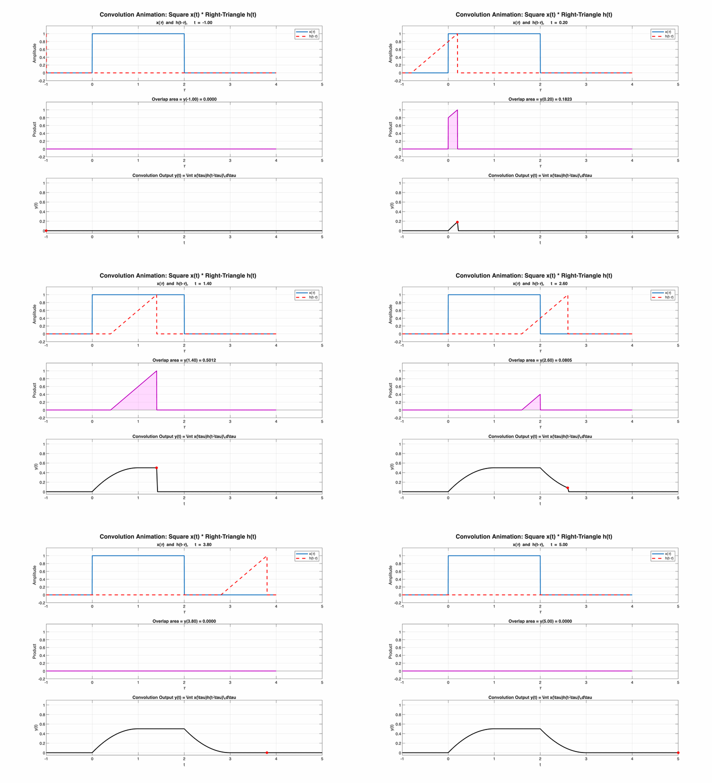
The animations below turn the convolution equations into a picture. First watch the shifted response move across the input. Next, look at the overlap in the middle panel. Its area (continuous time) or sum (discrete time) gives one output value. Repeating this process for every shift builds the complete output signal. Select Show full script if you want to see how MATLAB generates and exports the frames.
![Animation of discrete-time convolution: h[n0-m] sliding across x[m], with the sum of overlap stems tracing out y[n]](assets/conv_discrete.gif)
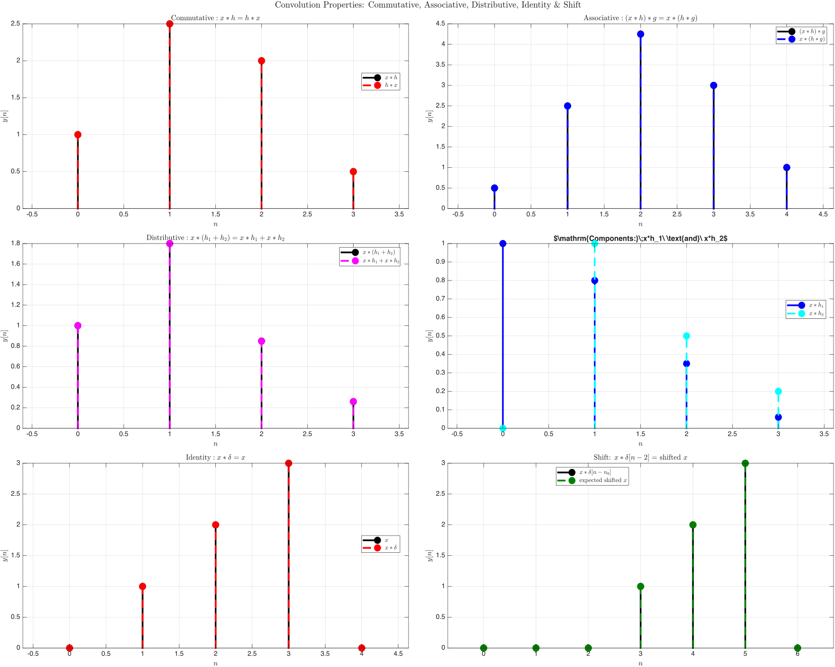
This script checks the properties from Section 1.3.2 with short test sequences. For each property, MATLAB calculates the left- and right-hand sides separately and overlays the results. Matching plots provide a numerical check of the algebra. The script also reports a value of 1 when each comparison passes.
?1.5 Problems with solutions
Try each problem before opening the solution. Write down the definition or property you plan to use first; this makes it easier to find where an incorrect solution went wrong.
1.6 Summary and key formulas
Use this reference sheet to review the classification tests, convolution formulas and four main convolution properties.
- Signals and systems are classified along recurring axes: periodic/aperiodic, causal/non-causal, energy/power (every periodic signal is a power signal), and even/odd (every signal splits uniquely into both parts).
- A system is linear if superposition holds (Eq. 1.8) and time-invariant if a shifted input produces an identically shifted output; together these define an LTI/LSI system.
- An LTI/LSI system is fully characterized by its impulse response \(h(t)\)/\(h[n]\): sifting the input into scaled, shifted impulses and pushing each through the system derives the convolution sum/integral above (Eq. 1.14, 1.15) as its output.
- Convolution's four properties, above, are exactly what let cascaded and parallel LTI/LSI systems be freely redrawn as a single equivalent system.
- Next, in Lecture 2: the Laplace transform, transfer functions, poles, zeros and stability, then the full Fourier ladder (CTFT, CTFS, DTFT, DTFS, DFT and the FFT) that filter design (Lectures 5–8) puts to work.