ELEC6218 · Signal Processing Analog & Digital Filter Design
Signal Processing · Lecture notes Prof. Çelik
ELEC6218 · Signal Processing
Lecture 3

Sampling and Reconstruction

How does a continuous signal become a sequence of numbers? We separate the process into sampling and quantization. Sampling can be reversed when the Nyquist condition is satisfied; quantization always introduces some error. Understanding that difference is essential for practical DSP.

Quiz
Podcast
InstructorProf. Abdulkadir Çelik (https://akadircelik.com) ModuleELEC6218 TopicsImpulse-train sampling · Nyquist · aliasing · sinc interpolation · ZOH · quantization & SQNR
▸ Spectral replication ▸ The Nyquist criterion ▸ Perfect reconstruction ▸ Quantization noise
Learning outcomes

By the end of this lecture, you will be able to:

  • Explain ideal sampling with an impulse train, show why sampling creates repeated copies of the spectrum, and use the Nyquist–Shannon theorem to calculate alias frequencies.
  • Convert between frequency in hertz \(f\), rad/s \(\Omega\), and rad/sample \(\omega\), and explain how sinc interpolation reconstructs a band-limited signal exactly in theory.
  • Explain why an anti-aliasing filter must come before the ADC, describe the zero-order hold's high-frequency droop, and show how oversampling relaxes analog filter requirements.
  • Estimate quantization noise and SQNR, use the 6 dB-per-bit rule, and relate a digital filter's response to the equivalent continuous-time response between an ADC and DAC.
Lecture 3

Contents

Sections 3.1–3.5 are the theory of sampling, and they are exact: nothing is lost. Sections 3.7–3.8 are what it costs to build, and there everything is an approximation. Section 3.13 collects the payoff.

iNotation used in this lecture
\(x_c(t)\)
the continuous-time signal at the input of the ADC
\(x_s(t)\)
the impulse-train-sampled signal (still continuous-time)
\(x[n]=x_c(nT)\)
the sequence handed to the DSP
\(T\), \(f_s=1/T\)
sampling period (s) and sampling rate (Hz)
\(\Omega_s=2\pi/T\)
sampling frequency in rad/s
\(\Omega_N\)
the highest frequency present in \(x_c(t)\) — the Nyquist frequency; \(2\Omega_N\) is the Nyquist rate
\(h_r(t)\), \(H_r(j\Omega)\)
the reconstruction (interpolation) filter
\(R\), \(\Delta\)
quantizer word length in bits, and step size
\(e[n]\), \(\sigma_e^2\)
quantization error sequence and its variance (noise power)

Keep the three frequency symbols separate. \(f\) is measured in hertz (cycles per second). \(\Omega=2\pi f\) is continuous-time angular frequency in rad/s. \(\omega=\Omega T\) is discrete-time frequency in rad/sample, where only one interval, usually \((-\pi,\pi]\), contains distinct frequencies. Always check the symbol and unit before substituting values.

3.1  The bridge: two different approximations, one signal chain

Sensors such as microphones, strain gauges, antennas and thermocouples produce a continuous-time signal \(x_c(t)\). A computer cannot store a value at every instant or represent every possible amplitude exactly. The signal must therefore be converted into a sequence of numbers.

This conversion has two separate stages. Understanding their difference is central to the lecture:

Discretising time · sampling

Potentially reversible. If the Nyquist condition is satisfied, the original band-limited signal can be reconstructed exactly from its samples. If the condition is violated, aliasing causes permanent information loss.

Discretising amplitude · quantization

Irreversible. Rounding \(2.7183\ldots\) to the nearest of \(2^R\) levels destroys the remainder permanently. There is no condition that makes it lossless; you can only make the loss small and predictable. Section 3.9.

Students routinely blur the two into “digitising”. Keeping them apart explains almost every practical decision an engineer makes here: you choose \(f_s\) to satisfy a hard constraint, and you choose \(R\) to hit a noise budget.

Anti-alias filter (LPF) Sample & hold Quantize + encode Digital filter DAC Zero-order hold Reconstr. filter (LPF) analog in x[n] analog out ADC — §3.2–3.4, §3.8 DAC — §3.6–3.7 Everything left of x[n] is Lecture 3. Everything to its right in the DSP block is Lectures 4–8.
Figure 3.1. The whole chain, and where each section of this lecture sits on it. Note the symmetry: the analog low-pass filter appears twice, once as an anti-aliasing filter guarding the entrance and once as a reconstruction filter guarding the exit. They do the same job (keep everything below \(f_s/2\)) for opposite reasons, and Section 3.8 explains why neither can be omitted.

3.2  Ideal sampling: multiplication by an impulse train

To analyse sampling we need a model of it that the Lecture 2 toolkit can act on. The trick, and it is only a trick, is to write sampling as a multiplication. Define the impulse train (the “Dirac comb”)

$$ s(t)=\sum_{n=-\infty}^{\infty}\delta(t-nT), $$
(3.1)

and form the product with the signal. The sifting property of Lecture 1 (\(x(t)\delta(t-t_0)=x(t_0)\delta(t-t_0)\)) then does the rest, turning a product of two awkward objects into a tidy weighted train:

$$\boxed{\;x_s(t)=x_c(t)\,s(t)=\sum_{n=-\infty}^{\infty}x_c(nT)\,\delta(t-nT).\;}$$
(3.2)

Each impulse carries an area equal to the signal's value at that instant. Two cautions, both worth stating because the notation invites confusion.

  • \(x_s(t)\) is still continuous-time. It is a function of \(t\) that happens to be zero except at multiples of \(T\). This is exactly what makes it useful: the CTFT of Lecture 2 can be applied to it, whereas it cannot be applied to a sequence.
  • \(x[n]\) is not \(x_s(t)\). The sequence \(x[n]=x_c(nT)\) is indexed on an integer and has been time-normalised: it has forgotten \(T\) entirely. The spacing between consecutive values of \(x[n]\) is always 1, never \(T\) seconds. Section 3.6 shows that this forgetting is exactly what rescales the frequency axis.

This is an ideal mathematical model, not a literal circuit. Real samplers use a switch with a short but finite aperture and hold the measured voltage on a capacitor; they do not generate Dirac impulses. The impulse-train model is still valuable because it predicts the correct frequency-domain effects in a simple form.

C/D converter xc(t) s(t) xₛ(t) conversion from impulse train to a sequence x[n] = xc(nT) (a) T = T₁−4T−2T02T4T······xₛ(t) T = 2T₁−2T−T0T2T······xₛ(t) (b) −4−3−2−101234x[n]n −2−1012x[n]n (c)
Figure 3.2. The two-stage model: impulse-train modulation, then conversion to a sequence. The middle row shows \(x_s(t)\) at two sampling rates, with arrow lengths proportional to impulse area; the bottom row shows the resulting \(x[n]\). Notice what changes and what does not: halving the rate visibly changes \(x_s(t)\) (the impulses move apart on a real time axis), but the two \(x[n]\) plots are drawn on the same integer axis. The sequence has no memory of \(T\).

3.3  What sampling does to a spectrum: replication

Now cash in the model. Eq. (3.2) is a product in time, and Lecture 2's Eq. (2.30) says a product in time is a convolution in frequency. We need one ingredient: the CTFT of the impulse train, which is itself an impulse train, spaced by the sampling frequency \(\Omega_s=2\pi/T\):

$$ S(j\Omega)=\frac{2\pi}{T}\sum_{k=-\infty}^{\infty}\delta(\Omega-k\Omega_s). $$
(3.3)

Because the sampling impulse train is periodic with period \(T\), its spectrum contains impulses at multiples of \(\Omega_s=2\pi/T\). Convolution with one shifted impulse creates one shifted copy of the original spectrum; convolution with the full train therefore creates repeated copies:

$$\boxed{\;X_s(j\Omega)=\frac{1}{2\pi}\,X_c(j\Omega)*S(j\Omega)=\frac{1}{T}\sum_{k=-\infty}^{\infty}X_c\big(j(\Omega-k\Omega_s)\big).\;}$$
(3.4)
The one sentence to take from this lecture

Sampling in time replicates the spectrum in frequency, every \(\Omega_s\), scaled by \(1/T\). Nothing is added and nothing is removed — the original spectrum is still there, sitting at \(k=0\), surrounded by an infinite queue of identical copies.

Equation (3.4) explains physically why a discrete-time spectrum is periodic. Sampling in time creates spectral copies separated by \(\Omega_s\). After the frequency axis is normalized, those copies repeat every \(2\pi\) rad/sample.

Everything that follows is a consequence of one question: do the copies overlap?

3.4  The Nyquist–Shannon theorem, and aliasing

Assume \(x_c(t)\) is band-limited, so \(X_c(j\Omega)=0\) for \(|\Omega|\ge\Omega_N\). The original spectrum has total width \(2\Omega_N\), and sampling places a copy at every multiple of \(\Omega_s\). The original and its nearest copy do not overlap when

$$\boxed{\;\Omega_s-\Omega_N\ \ge\ \Omega_N \quad\Longleftrightarrow\quad \Omega_s\ \ge\ 2\Omega_N \quad\Longleftrightarrow\quad f_s\ \ge\ 2f_N.\;}$$
(3.5)
The Nyquist–Shannon sampling theorem

Let \(x_c(t)\) be band-limited with \(X_c(j\Omega)=0\) for \(|\Omega|\ge\Omega_N\). Then \(x_c(t)\) is uniquely determined by its samples \(x[n]=x_c(nT)\), \(n\in\mathbb{Z}\), provided \(\Omega_s=2\pi/T\ge2\Omega_N\).

\(\Omega_N\) is the Nyquist frequency (a property of the signal); \(2\Omega_N\) is the Nyquist rate (the requirement on the sampler). The two are constantly confused; the rate is the one you compare \(f_s\) against.

The theorem says more than “the samples are a good approximation.” For a band-limited signal sampled above the Nyquist rate, the samples determine the continuous waveform exactly, including every value between sampling instants. Band-limiting is essential because it restricts how quickly the waveform can change.

Ω1−ΩₙΩₙXc(jΩ)(a) Ω−2Ωₛ−Ωₛ0Ωₛ2ΩₛS(jΩ)2π/T(b) Ω1/T(Ωₛ−Ωₙ) − Ωₙ ≥ 0Xₛ(jΩ)(c) Ωₛ ≥ 2Ωₙ — no aliasing ΩXₛ(jΩ)(Ωₛ−Ωₙ) < Ωₙ ⇒ replicas add(d) Ωₛ < 2Ωₙ — aliasing
Figure 3.4.a. Eq. (3.4) drawn. (a) the band-limited original, (b) the sampling comb, (c) \(\Omega_s\ge2\Omega_N\): the replicas are separated by a clear gap, so the \(k=0\) copy can be cut out intact and the original recovered exactly. (d) \(\Omega_s<2\Omega_N\): the replicas overlap and are added together by Eq. (3.4). The sum in the overlap region is a new spectrum that no filter can unmix — you cannot separate two numbers once you have only their total.

3.4.1  Where the factor of two comes from

The factor of two follows directly from the spectral copies in Eq. (3.4). Each copy extends from \(-\Omega_M\) to \(+\Omega_M\) around its centre, so its total width is \(2\Omega_M\).

The replica centred at \(\Omega=0\) extends up to \(+\Omega_M\). Its neighbour, centred at \(\Omega_s\), extends down to \(\Omega_s-\Omega_M\). They stay clear of each other precisely when

$$\Omega_s - \Omega_M > \Omega_M \quad\Longleftrightarrow\quad \Omega_s > 2\Omega_M \quad\Longleftrightarrow\quad f_s > 2f_M.$$
(3.6)

The replicas must therefore be separated by at least \(2\Omega_M\). The detailed shape of the spectrum does not matter for this baseband result; only its highest occupied frequency matters.

When the condition holds, the baseband copy sits alone in \(|\Omega|<\Omega_s-\Omega_M\), so an ideal lowpass filter isolates it exactly, and the \(1/T\) in Eq. (3.4) is undone by a gain of \(T\):

$$X(j\Omega) = T\,H_r(j\Omega)\,X_s(j\Omega), \qquad H_r(j\Omega)=\begin{cases}1,&|\Omega|<\Omega_c\\0,&\text{otherwise}\end{cases}, \qquad \Omega_M < \Omega_c < \Omega_s-\Omega_M.$$
(3.7)

Equation (3.7) shows two useful results. First, reconstruction is exact when the Nyquist condition is satisfied. Second, the reconstruction-filter cutoff may lie anywhere between the original spectrum and its nearest copy. This empty region is the guard band. Sampling exactly at the Nyquist rate leaves no guard band, while oversampling makes practical filter design easier by widening it.

3.4.2  Aliasing: where the energy actually goes

“The replicas overlap” is geometrically clear but does not yet tell you what you will hear. Take the simplest possible signal, a cosine at \(\Omega_0\), whose spectrum is one impulse pair at \(\pm\Omega_0\) (Section 2.9.1). Sample it and Eq. (3.4) puts a pair at \(\pm\Omega_0+k\Omega_s\) for every \(k\). Now reconstruct with an ideal low-pass cutting at \(\Omega_s/2\), and ask which line survives:

  • \(\Omega_0<\Omega_s/2\). The \(k=0\) pair is inside the cutoff and every other pair is outside. Out comes \(\cos(\Omega_0 t)\). Correct.
  • \(\Omega_s/2<\Omega_0<\Omega_s\). Now the \(k=0\) pair is outside the cutoff and gets discarded — but the \(k=-1\) pair, sitting at \(\Omega_0-\Omega_s\), has moved inside it. Out comes a cosine at a frequency that was never in the input:
$$ x_r(t)=\cos\big((\Omega_s-\Omega_0)\,t\big). $$
(3.8)

The high tone has taken on the alias of a lower one. Geometrically the frequency has been folded about \(\Omega_s/2\), which is why \(f_s/2\) is also called the folding frequency: \(f_s/2+\varepsilon\) comes back as \(f_s/2-\varepsilon\). This is the frequency-domain twin of Lecture 2's Problem 2.3 — there, two cosines produced an identical sequence; here we see which of them a reconstructor will pick, and it always picks the one below \(f_s/2\).

(a) Ω₀ < Ωₓ/2 — no aliasing: the k=0 pair is inside the band +Ωₓ/2 −Ωₓ/2 −Ω₀ +Ω₀ (b) Ωₓ/2 < Ω₀ < Ωₓ — aliasing: the tone folds back inside the band +Ωₓ/2 −Ωₓ/2 Ω₀ (discarded) Ωₓ−Ω₀
Figure 3.4.b. Aliasing of a single cosine, in the frequency domain. Solid stems are the lines that fall inside the reconstruction filter's passband and therefore appear at the output; dashed stems are replicas that are filtered away. In (b) the roles have swapped: the genuine line is rejected and a replica is admitted in its place. The reconstructor is not malfunctioning — the samples are genuinely consistent with both tones, and it returns the only one it is allowed to.
Aliasing cannot be fixed later

Once spectral replicas overlap, their values add and the original contributions cannot be separated. An aliased component looks exactly like a genuine component at the same frequency; it is not a removable noise layer. The protection must therefore come before sampling. An analog anti-alias filter removes frequencies that would fold into the wanted band, which is why it appears before the ADC in Figure 3.1.

EXAMPLE 3.1 · Two different signals, one identical sequence

Sample \(x_c(t)=\cos(4000\pi t)\) and \(\tilde{x}_c(t)=\cos(16000\pi t)\), both with \(T=1/6000\,\text{s}\). Compare the sequences, and say what an ideal reconstructor returns in each case.

Step 1. Here \(\Omega_s=2\pi/T=12000\pi\), so the folding frequency is \(\Omega_s/2=6000\pi\).

Step 2 · First signal. \(\Omega_0=4000\pi<6000\pi\), so Nyquist is satisfied. By Eq. (3.13), \(\omega_0=\Omega_0T=4000\pi/6000=2\pi/3\), comfortably inside \((-\pi,\pi]\), and

$$x[n]=\cos(2\pi n/3).$$

Step 3 · Second signal. \(\tilde\Omega_0=16000\pi>6000\pi\): Nyquist is violated. But watch what the samples do:

$$\tilde{x}[n]=\cos\!\left(\frac{16000\pi n}{6000}\right)=\cos\!\left(2\pi n+\frac{4000\pi n}{6000}\right)=\cos(2\pi n/3).$$

The two sequences are identical, number for number. Nothing in \(x[n]\) records which signal produced it.

Step 4 · Reconstruction. Both return \(\cos(4000\pi t)\) — correct for the first signal, and for the second the alias predicted by Eq. (3.8): \(\Omega_s-\tilde\Omega_0=12000\pi-16000\pi=-4000\pi\), i.e. \(4000\pi\) by evenness. The \(8\,\text{kHz}\) tone has come back as \(2\,\text{kHz}\). This is Lecture 2's Problem 2.3 with physical units attached, and it shows why aliasing is irreversible: the information was destroyed at the sampler, not at the reconstructor.

EXAMPLE 3.2 · The wagon-wheel effect, quantitatively

A camera films at \(24\,\text{frames/s}\) a wheel with 12 spokes rotating at \(2\,\text{rev/s}\). What does the film show?

Step 1. The camera is a sampler with \(f_s=24\,\text{Hz}\), so the folding frequency is \(12\,\text{Hz}\). The observable signal is not the wheel's rotation but the passage of spokes, since consecutive spokes are indistinguishable:

$$f_{\text{spoke}}=12\ \text{spokes}\times 2\ \text{rev/s}=24\ \text{Hz}.$$

Step 2. \(24>12\), so Nyquist is violated. By Eq. (3.8) the apparent frequency is \(|f_s-f_0|=|24-24|=0\,\text{Hz}\): the wheel appears stationary while the wagon moves.

Step 3. Speed it up slightly to \(2.1\,\text{rev/s}\) and \(f_{\text{spoke}}=25.2\,\text{Hz}\), aliasing to \(|24-25.2|=1.2\,\text{Hz}\) — the wheel now appears to creep forward slowly. Slow it to \(1.9\,\text{rev/s}\) and \(f_{\text{spoke}}=22.8\,\text{Hz}\) aliases to \(1.2\,\text{Hz}\) as well, but on the other side of the fold, so the wheel appears to turn backwards. A cinema screen is a sampling system with no anti-aliasing filter, and this is the resulting artefact.

MATLAB corner

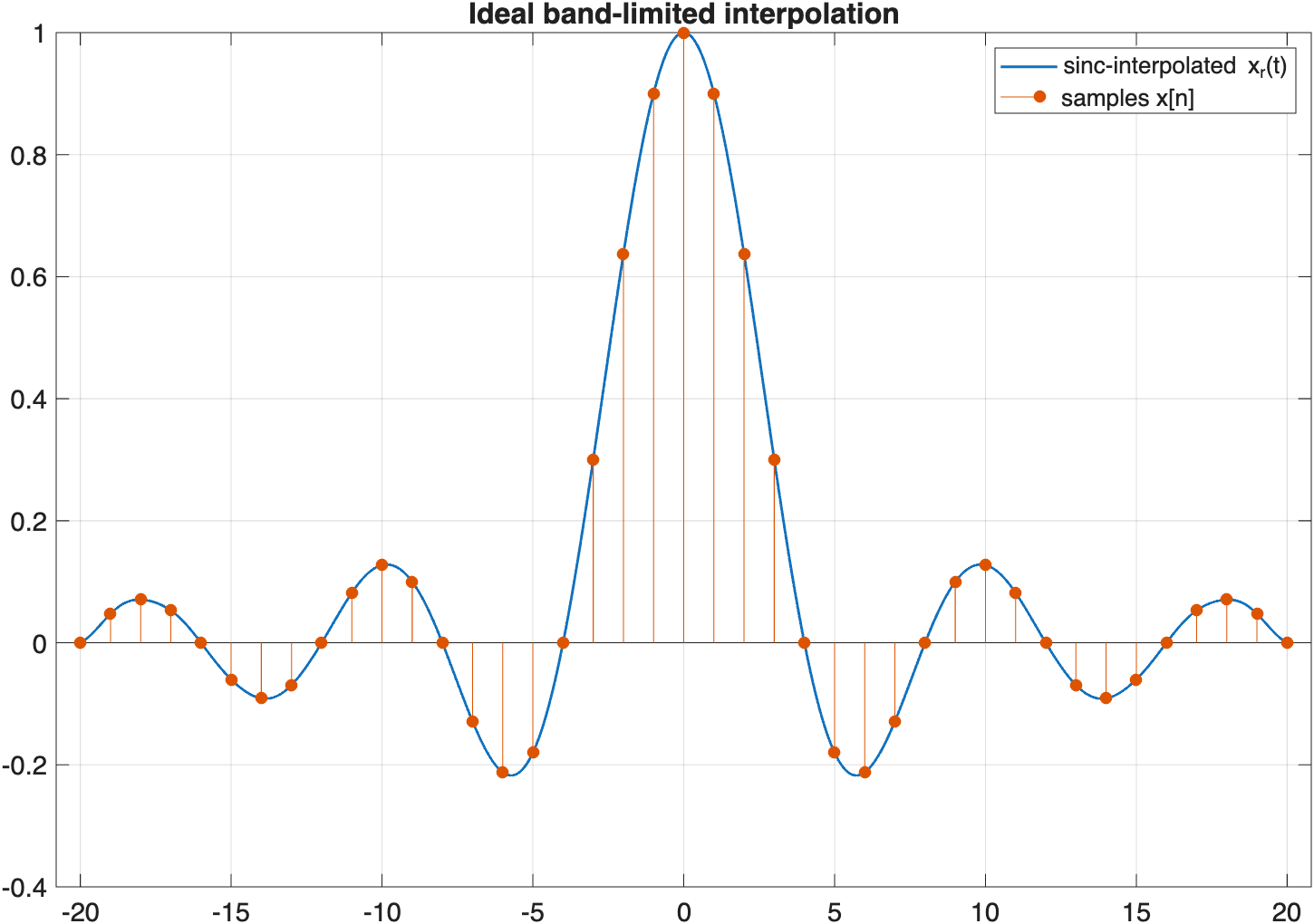
This script gives three views of sampling. First, it sweeps a tone through the Nyquist frequency and measures the alias that appears in the sampled data. Next, it plays the same folding effect as a chirp. Finally, it uses Eq. (3.17) to reconstruct a band-limited signal and checks that the sinc interpolation passes through every sample.

Goal: plot measured vs. true frequency through and past \(f_s/2\) to see the fold happen numerically, then verify ideal sinc interpolation reconstructs the samples exactly.

aliasing_demo.m
MATLAB
%% aliasing_demo.m - Part 1: watch a tone fold back about fs/2  (Eq. 3.6)
fs = 1000;                       % sampling rate, so folding is at 500 Hz
f0 = 100:50:1900;                % sweep the true tone well past fs/2
n  = 0:2047;
fa = zeros(size(f0));
for k = 1:numel(f0)
    x = cos(2*pi*f0(k)/fs*n);    % the SAMPLES - all we ever get
    X = abs(fft(x .* hann(numel(n))'));
    [~,i] = max(X(1:end/2));
    fa(k) = (i-1)*fs/numel(n);   % frequency actually measured
end
figure('Color','w'); plot(f0, fa, 'LineWidth', 1.6); grid on; hold on;
plot(f0, f0, '--'); xline(fs/2, 'r:', 'f_s/2'); xline(fs, 'r:', 'f_s');
xlabel('true frequency (Hz)'); ylabel('measured frequency (Hz)');
title('The triangle wave of aliasing: everything folds into [0, f_s/2]');
% -> rises to 500, folds back to 0 at 1000, rises again... forever.
%% Part 2 - the same thing you can HEAR (needs a sound card)
fsa = 8000; t = 0:1/fsa:3;
chirp_true = chirp(t, 0, 3, 12000);   % sweeps up to 12 kHz > fsa/2 = 4 kHz
soundsc(chirp_true, fsa);
% The pitch rises, hits 4 kHz, then falls again - it cannot exceed fs/2.
%% Part 3 - sinc interpolation really does pass through every sample
T = 1; n = -20:20; x = sinc(n/4);   % a band-limited test sequence
t = linspace(-20, 20, 4000);
xr = zeros(size(t));
for k = 1:numel(n)
    xr = xr + x(k) * sinc((t - n(k)*T)/T);   % Eq. (3.17)
end
figure('Color','w'); plot(t, xr, 'LineWidth', 1.4); hold on; grid on;
stem(n, x, 'filled');
legend('sinc-interpolated x_r(t)', 'samples x[n]');
title('Ideal band-limited interpolation');
Measured frequency versus true frequency: a triangle wave folding everything into [0, fs/2] Ideal band-limited interpolation: a sinc-interpolated waveform passing through every sample
Figure 3.4.c. Reading the two MATLAB plots. In the left plot, the measured frequency follows the true frequency only up to \(f_s/2\). It then folds back towards zero, rises again, and repeats. The samples therefore never identify a frequency above the Nyquist limit directly; they report an alias inside \([0,f_s/2]\). In the right plot, the sinc reconstruction passes through every sample marker. Each sinc term is zero at the other sample positions, so their sum preserves the given samples while filling in the values between them.

3.4.3  The general folding rule, and the strobe

Example 3.2 worked three cases of one wheel by folding each spoke frequency against \(f_s\) by hand. The rule behind all three is worth stating once, because it applies to any periodic motion under any sampler: the observer reconstructs the smallest motion consistent with the samples, so the apparent rate is the true rate folded into \(|f|\le f_s/2\):

$$f_a = f_r - f_s\left\lceil\frac{f_r}{f_s}-\frac{1}{2}\right\rfloor, \qquad |f_a| \le \frac{f_s}{2},$$
(3.9)

where \(\lceil\cdot\rfloor\) rounds to the nearest integer. The consequences are the ones everyone has seen. At \(f_r=f_s\) the wheel advances exactly one full turn between frames and appears frozen. Just below \(f_s\) it falls slightly short each frame, so \(f_a\) is negative and the wheel appears to turn backwards. Just above, it creeps slowly forwards. None of this is an artefact of film or of the eye: it is Eq. (3.8) with a rotation in place of a sinusoid.

f_r = 0.25 f_s↻ appears forward f_r = f_s— appears frozen f_r = 0.92 f_s↺ appears reversed
Figure 3.4.d. Three spoke positions from three consecutive frames, for one wheel at three rotation rates. Sampling below the Nyquist rate does not blur the motion, it reports a different motion — and reports it just as confidently.

One consequence is worth naming, because it is the basis of an instrument and of a recurring mistake. A strobe flashing at \(f_s\) freezes a shaft turning at \(f_r\) whenever \(f_a=0\), which happens not only at \(f_r=f_s\) but at every \(f_r=kf_s\). A stationary image therefore fixes the shaft speed only up to an unknown integer \(k\), and a strobe tachometer read at the first frozen image can be wrong by an exact multiple. The standard procedure — halve the flash rate and check whether the image freezes again — is Eq. (3.9) being used to resolve \(k\).

3.5  Undersampling on purpose: when \(f_s<2f_{\max}\) is legitimate

Section 3.4 is routinely misquoted as "sample at twice the highest frequency". What Eq. (3.6) actually requires is that the replicas do not overlap, and for a signal whose energy occupies a band well away from zero, that is a much weaker requirement than twice the highest frequency. Exploiting the difference is called bandpass sampling, or undersampling, and it is standard practice in radio receivers.

Let the signal occupy \(f_L \le |f| \le f_H\), with bandwidth \(B = f_H - f_L\). Sampling still places replicas at every multiple of \(f_s\), but the band and its mirror image now have gaps between them for the replicas to land in. Non-overlap holds when \(f_s\) is chosen from one of a set of allowed windows:

$$\frac{2f_H}{n} \;\le\; f_s \;\le\; \frac{2f_L}{n-1}, \qquad n = 1,2,\dots,\left\lfloor \frac{f_H}{B} \right\rfloor.$$
(3.10)

Each \(n\) is a Nyquist zone: the band folds down to baseband from the \(n\)-th zone up. Taking the largest admissible \(n\) gives the lowest usable rate,

$$f_{s,\min} = \frac{2f_H}{\lfloor f_H/B \rfloor} \;\ge\; 2B,$$
(3.11)

so the true floor is twice the bandwidth, not twice the top frequency, and it is reached only when \(f_H\) happens to be an integer multiple of \(B\). Note that \(n=1\) recovers ordinary baseband sampling, \(f_s \ge 2f_H\), so Eq. (3.10) contains the Nyquist rule rather than contradicting it.

f signal band, B f_L f_H replica replicas land in the gaps — no overlap, so nothing is lost f_s 2f_s 3f_s 4f_s sampling at f_s ≪ 2f_H folds the band down to baseband intact
Figure 3.5. A band well away from DC, sampled far below \(2f_H\). The replicas interleave with the original band instead of overlapping it, so one of them lands cleanly at baseband and the signal survives. Choose \(f_s\) badly and the same picture shows replicas on top of each other.

What undersampling does not buy you. The rate requirement falls; three other requirements do not. The anti-aliasing filter must now be a bandpass filter sharp enough to remove everything outside \(f_L\!\ldots\!f_H\), since out-of-band noise from every zone folds down on top of the signal. The converter's analogue input bandwidth and sample-and-hold aperture must still reach \(f_H\) — a converter clocked at \(8\) MHz cannot necessarily see a \(72\) MHz input. And clock jitter is now weighted by \(f_H\), not by \(f_s\), so the jitter specification tightens by exactly the factor you saved.

EXAMPLE 3.3 · Sampling a 70 MHz IF

A receiver presents an intermediate-frequency signal spanning \(68\)–\(72\) MHz to an ADC. Baseband sampling would need \(f_s > 144\) MHz. Find the admissible sampling rates, and the lowest one.

Step 1. \(f_L = 68\) MHz, \(f_H = 72\) MHz, so \(B = 4\) MHz and \(\lfloor f_H/B \rfloor = \lfloor 18 \rfloor = 18\). There are 18 Nyquist zones to choose from.

Step 2. Applying Eq. (3.10) for a few values of \(n\):

nlower limit 2f_H/nupper limit 2f_L/(n−1)window
1014.40 MHz15.11 MHz0.71 MHz wide
169.00 MHz9.07 MHz0.07 MHz wide
188.00 MHz8.00 MHza single point

Step 3. The lowest rate is \(f_{s,\min} = 2(72)/18 = 8\) MHz, exactly \(2B\) — achievable here only because \(f_H\) is an exact multiple of \(B\). It is also a single admissible value with no tolerance, so a real design would not use it.

Step 4. A sensible choice is \(n=10\), \(f_s = 14.7\) MHz: still a tenth of the baseband rate, but with \(0.7\) MHz of clock tolerance either side. The ADC must nonetheless accept a \(72\) MHz input and be clocked with jitter budgeted against \(72\) MHz, per the note above.

3.6  The exchange rate: \(\omega=\Omega T\), and the debt from Lecture 2

Lecture 2's glossary promised that Lecture 3 would supply the conversion between continuous-time frequency and discrete-time frequency. It falls out of two lines. Take the CTFT of the impulse train in Eq. (3.2), using the sifting property to evaluate each integral:

$$ X_s(j\Omega)=\sum_{n=-\infty}^{\infty}x_c(nT)\!\!\int_{-\infty}^{\infty}\!\!\delta(t-nT)e^{-j\Omega t}dt = \sum_{n=-\infty}^{\infty}x_c(nT)\,e^{-j\Omega Tn}. $$
(3.12)

Set that beside the DTFT of the sequence, Eq. (2.40), \(X(e^{j\omega})=\sum_n x[n]e^{-j\omega n}\). With \(x[n]=x_c(nT)\), the two sums are term by term identical the moment we identify \(\omega\) with \(\Omega T\):

$$\boxed{\;X_s(j\Omega)=X(e^{j\omega})\big|_{\omega=\Omega T}, \qquad \omega=\Omega T=\frac{\Omega}{f_s}=\frac{2\pi f}{f_s}.\;}$$
(3.13)

The CTFT of the sampled signal and the DTFT of the sequence are the same function, drawn on two differently labelled axes. Substituting into Eq. (3.4) gives the relation in the form you will use most often:

$$ X(e^{j\omega})=\frac{1}{T}\sum_{k=-\infty}^{\infty}X_c\!\left(j\left(\frac{\omega}{T}-\frac{2\pi k}{T}\right)\right). $$
(3.14)

Once the signal is written as \(x[n]\), the physical time interval \(T\) is no longer visible on the sample index. The frequency axis must therefore be normalized by the sampling rate. This gives the conversion

DC
\(\Omega=0 \ \longleftrightarrow\ \omega=0\)
Folding frequency
\(\Omega=\Omega_s/2 \ \longleftrightarrow\ \omega=\pi\)
One full replica
\(\Omega=\Omega_s \ \longleftrightarrow\ \omega=2\pi\)

The sampling frequency \(f_s\) maps to \(2\pi\) rad/sample, so the spectral copies repeat every \(2\pi\) on the discrete-time axis. The Nyquist frequency \(f_s/2\) maps to \(\omega=\pi\). Thus, DTFT periodicity and the folding of analog frequencies around \(f_s/2\) are two descriptions of the same effect.

Worked conversion · keep this to hand

A \(1\,\text{kHz}\) tone sampled at \(f_s=8\,\text{kHz}\):

Hz
\(f=1000\)
rad/s
\(\Omega=2\pi f=6283\)
rad/sample
\(\omega=\Omega T=2\pi(1000)/8000=\pi/4\)
check
\(\pi/4<\pi\) ✓ — below folding, so no aliasing

The shortcut worth memorising: \(\omega/\pi\) is the fraction of the way to \(f_s/2\). Here \(0.25\), i.e. a quarter of the way to the folding frequency. MATLAB's filter-design functions take exactly this normalised number.

3.7  Reconstruction: the ideal filter and sinc interpolation

Figure 3.4.a(c) already contains the recipe: if the replicas do not overlap, keep the one at \(k=0\) and throw the rest away. That is a low-pass filter. Its gain must be \(T\) to undo the \(1/T\) in Eq. (3.4), and its cutoff \(\Omega_c\) may sit anywhere in the gap:

$$ H_r(j\Omega)=\begin{cases}T, & |\Omega|\le\Omega_c\\ 0, & |\Omega|>\Omega_c\end{cases} \qquad \Omega_N\le\Omega_c\le\Omega_s-\Omega_N. $$
(3.15)

The usual choice is \(\Omega_c=\Omega_s/2=\pi/T\), which is legal for any rate satisfying Eq. (3.5). Now translate to the time domain. A rectangle in frequency inverts to a sinc in time — Lecture 2's Section 2.9.1, read right to left — so

$$ h_r(t)=\frac{\sin(\pi t/T)}{\pi t/T}, \qquad h_r(0)=1,\quad h_r(nT)=0\ \ (n\ne0). $$
(3.16)

Filtering the impulse train of Eq. (3.2) means convolving with \(h_r\), and convolving an impulse train just drops a copy of \(h_r\) at each impulse, weighted by its area. The result is the Whittaker–Shannon interpolation formula:

$$\boxed{\;x_r(t)=\sum_{n=-\infty}^{\infty}x[n]\,\frac{\sin\!\big[\pi(t-nT)/T\big]}{\pi(t-nT)/T}.\;}$$
(3.17)

At a sampling instant \(t=mT\), the sinc for sample \(m\) equals 1 and every other sinc equals 0. The reconstructed curve therefore passes exactly through every sample. Between sample instants, many sinc terms contribute. The Nyquist condition determines whether those in-between values reproduce the original signal or an aliased alternative.

ideal reconstruction system x[n] sequence → impulse train xₛ(t) ideal reconstruction filter Hᵣ(jΩ) xᵣ(t) sampling period T (a) Ω T −π/T π/T Hᵣ(jΩ) (b) 1 −4T−3T−2T−TT2T3T4T 0 hᵣ(t) = sin(πt/T)/(πt/T) t (c)
Figure 3.7. Sinc interpolation in action. The bottom panel shows several individual terms \(x[n]h_r(t-nT)\) of Eq. (3.17) and their sum. Each sinc is at its peak where its own sample sits and passes through zero at every other sample instant, so the terms never interfere at the sample points — they only fill in the gaps. “Connecting the dots” with straight lines is a crude approximation to this; the sinc is the exactly correct curve.
Exact, and unbuildable

Ideal sinc interpolation cannot be implemented exactly in real time. Each sinc extends from \(-\infty\) to \(+\infty\), so reconstruction at one instant would require every past and future sample. The impulse response is therefore non-causal and infinitely long.

This is the same time–frequency trade-off seen in Lecture 2: a perfect brick-wall response in frequency corresponds to an infinite sinc in time. Practical reconstruction and FIR filters approximate the sinc with finite, causal systems.

3.8  What real hardware does instead: AAF, ZOH, oversampling

3.8.1  The anti-aliasing filter, and why it must come first

Real signals are never perfectly band-limited. Noise and interference can extend well above the intended signal band, and these components will fold into the measurement when sampled.

An analog low-pass anti-aliasing filter is therefore placed before the sampler to remove unwanted high-frequency content. It cannot be replaced by a digital filter after the ADC, because aliasing has already mixed the frequencies by that stage and the original components can no longer be separated.

3.8.2  Oversampling: buying filter margin with sample rate

A real anti-aliasing filter needs a finite transition band between frequencies it passes and rejects. Sampling exactly at the Nyquist rate leaves no transition band and would require an unrealistically sharp analog filter.

Oversampling uses a sampling rate well above \(2f_N\). The spectral copies move farther apart, leaving more frequency space for a gradual analog roll-off. A simpler analog filter can then be followed by a sharp digital filter and decimation. This is why practical audio converters sample above 40 kHz for a 20 kHz audio band, and why sigma–delta converters often use much higher internal rates.

A second dividend: 3 dB per doubling

Oversampling also improves SNR, and Section 3.9 will explain why in one line: the quantization noise power \(\sigma_e^2\) is fixed by \(\Delta\) alone, but it is spread evenly over \((-\pi,\pi]\), i.e. over the whole band up to \(f_s/2\). Double \(f_s\) and the same total noise is spread over twice the bandwidth, so only half of it lands in your signal band. That is \(3\,\text{dB}\) per doubling — half a bit — free. Noise shaping in \(\Sigma\Delta\) converters improves the exchange rate dramatically further.

3.8.3  The zero-order hold, and its sinc droop

At the output end, a practical DAC does not emit impulses either. It emits the simplest thing a latch and a switch can produce: it holds each sample constant for a full period. This is the zero-order hold,

$$ x_{\text{ZOH}}(t)=\sum_{n=-\infty}^{\infty}x[n]\,\mathrm{rect}\!\left(\frac{t-nT}{T}\right), $$
(3.18)

which is exactly Eq. (3.17) with the sinc kernel replaced by a rectangle — the crudest possible interpolator, a staircase. Its cost is immediate from the \(\mathrm{rect}\leftrightarrow\mathrm{sinc}\) pair: the ZOH is an LTI filter whose frequency response is a sinc,

$$\boxed{\;H_{\text{ZOH}}(j\Omega)=T\,\mathrm{sinc}\!\left(\frac{\Omega T}{2}\right)e^{-j\Omega T/2}.\;}$$
(3.19)

The zero-order hold has two main effects. Its sinc-shaped magnitude response falls with frequency, reaching \(2/\pi=0.637\), or \(-3.9\,\text{dB}\), at \(f_s/2\); practical DAC systems often compensate for this droop. Its phase term \(e^{-j\Omega T/2}\) represents a delay of half a sample and does not distort the waveform shape. The sinc zeros at multiples of \(f_s\) also help suppress the spectral images.

coarse hold — T larget fine hold — T small (oversampled)t dashed: the band-limited signal; solid: what the ZOH actually emits
Figure 3.8. The zero-order hold: each sample held for \(T\) seconds, giving the familiar staircase. Compare with Figure 3.4.c — both interpolate through the samples, but the ZOH's rectangular kernel is a far blunter instrument than the sinc, and Eq. (3.19) is the bill for it.

3.9  Quantization: the loss that cannot be undone

Sampling handled the time axis. The amplitude axis is still continuous, and Section 3.1 warned that this half of the problem has no Nyquist theorem to rescue it. An \(R\)-bit quantizer maps each sample to the nearest of \(2^R\) levels spanning \([-X_m,X_m]\), so the step size is

$$ \Delta=\frac{2X_m}{2^{R}}=\frac{X_m}{2^{R-1}}. $$
(3.20)

Quantization is a non-linear, memoryless operation, which is bad news: none of the machinery of Lectures 1–2 applies to it. The standard escape is to stop treating it as an operation at all and model it as an added signal,

$$ \hat{x}[n]=x[n]+e[n], \qquad -\tfrac{\Delta}{2}\le e[n]\le \tfrac{\Delta}{2}, $$
(3.21)

and to assume \(e[n]\) is white, uniformly distributed, and uncorrelated with \(x[n]\). Under those assumptions the noise power is a one-line integral:

$$\boxed{\;\sigma_e^2=\mathbb{E}\!\left[e^2\right]=\int_{-\Delta/2}^{\Delta/2}\!\!\frac{e^2}{\Delta}\,de=\frac{\Delta^2}{12}.\;}$$
(3.22)
xc(t) C/D x[n] quantizer x̂[n] coder B[n] T −4Δ−3Δ−2Δ−ΔΔ−3Δ/2−Δ/2Δ/23Δ/2000001010011100101110111 x x̂ = Q(x) offset binary 2Xₘ full-scale range, 2ᴿ levels, step Δ 1/Δ −Δ/2 Δ/2 e pe(e) — assumed uniform σₑ² = ∫ e² pₑ(e) de = Δ²/12
Figure 3.9.a. The quantizer staircase and its error. The error is a deterministic sawtooth function of the input, bounded by \(\pm\Delta/2\) — which is exactly why calling it “noise” is a model, not a fact. It is a very good model when the signal is busy enough to traverse many levels between samples, and a poor one otherwise.

3.9.1  SQNR and the 6 dB-per-bit rule

Take a signal that uses the converter's full range, uniformly distributed on \([-X_m,X_m]\). Its power is \(P_x=\frac{1}{2X_m}\int_{-X_m}^{X_m}x^2dx=X_m^2/3\), and dividing by Eq. (3.22) with \(\Delta\) from Eq. (3.20):

$$ \mathrm{SQNR}=\frac{P_x}{\sigma_e^2}=\frac{X_m^2/3}{\Delta^2/12}=\frac{4X_m^2}{\Delta^2}=2^{2R}. $$
(3.23)
$$\boxed{\;\mathrm{SQNR}_{\text{dB}}=10\log_{10}2^{2R}\approx 6.02\,R\ \text{dB}.\;}$$
(3.24)

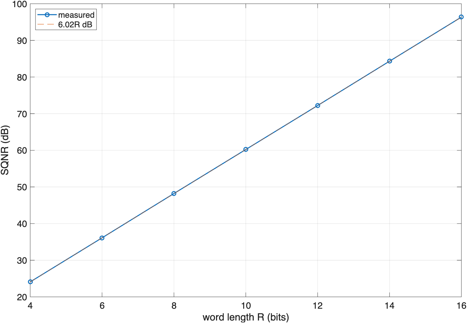
Each additional bit improves the ideal SQNR by about 6 dB. This gives approximately 48 dB for 8 bits, 72 dB for 12 bits, 96 dB for 16 bits and 144 dB for 24 bits. These values assume that the input uses the converter's full range. If the signal amplitude is halved, the SQNR falls by 6 dB, so correct input gain is important as well as bit depth.

When the white-noise model fails

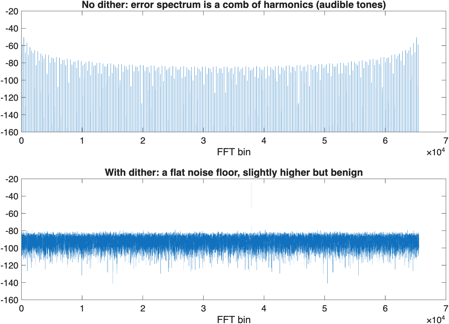
The white-noise model assumes that the quantization error is not correlated with the input. This assumption can fail for simple signals such as a slow ramp or a periodic sinusoid. The error then repeats in a structured pattern and creates harmonic tones rather than a smooth noise floor.

A small random signal called dither can be added before quantization. Dither breaks the correlation between the signal and the error, replacing tonal distortion with a slightly higher but smoother noise floor. It does not remove error power, but often makes the error less noticeable.

MATLAB corner

Equation (3.24) predicts how SQNR changes with word length. The script first tests that prediction using a signal that spans many quantizer levels. It then uses a low-level sinusoid to show when the usual additive-noise model becomes unreliable, and how dither changes the error.

Goal: measure SQNR vs. word length against the \(6.02R\) dB line, then show a low-level sinusoid's quantization error collapse into audible tones without dither.
quantization_sqnr.m
MATLAB
%% quantization_sqnr.m - measure the 6.02R dB rule instead of trusting it  (Eq. 3.24)
N = 2^16;  Xm = 1;
x = Xm * (2*rand(1,N) - 1);      % uniform on [-Xm, Xm], as Eq. (3.23) assumes
bits = 4:2:16;  sqnr = zeros(size(bits));
for k = 1:numel(bits)
    R = bits(k);
    D = Xm / 2^(R-1);                        % step size, Eq. (3.20)
    xq = D * round(x/D);                     % the quantizer
    e  = xq - x;
    sqnr(k) = 10*log10(mean(x.^2)/mean(e.^2));
    fprintf('R=%2d  measured %6.2f dB   var(e)=%.3e  D^2/12=%.3e\n', ...
            R, sqnr(k), var(e), D^2/12);
end
figure('Color','w'); plot(bits, sqnr, 'o-', 'LineWidth',1.5); hold on; grid on;
plot(bits, 6.02*bits, '--');
xlabel('word length R (bits)'); ylabel('SQNR (dB)');
legend('measured', '6.02R dB', 'Location','northwest');
% var(e) matches D^2/12 to ~1%: the model of Eq. (3.22) is sound HERE.
%% Now break the model: quantize a slow, low-level sinusoid
n = 0:N-1;  R = 6;  D = Xm/2^(R-1);
xs  = 0.02 * sin(2*pi*n/512);            % tiny signal, spans few levels
es  = D*round(xs/D) - xs;
xd  = xs + (rand(1,N)-0.5)*D;            % + 1 LSB of dither
ed  = D*round(xd/D) - xs;
figure('Color','w');
subplot(2,1,1); plot(20*log10(abs(fft(es.*hann(N)'))/N)); ylim([-160 -20]);
  title('No dither: error spectrum is a comb of harmonics (audible tones)');
subplot(2,1,2); plot(20*log10(abs(fft(ed.*hann(N)'))/N)); ylim([-160 -20]);
  title('With dither: a flat noise floor, slightly higher but benign');
Measured SQNR versus word length, lying on the 6.02R dB line Quantization error spectra: a comb of harmonics without dither, a flat noise floor with dither
Figure 3.9.b. What the MATLAB results mean. The measured SQNR rises by about \(6.02\,\text{dB}\) for each additional bit, closely following the theoretical line. This happens because one extra bit halves the quantization step and reduces the error power by roughly a factor of four. The error spectrum of a low-level sinusoid tells a second story: without dither, the error is correlated with the input and forms discrete harmonic peaks. With dither, those peaks spread into a more noise-like floor. Dither does not remove error power, but it makes the distortion less tonal and usually less audible.
EXAMPLE 3.4 · Designing the front end of an audio ADC

An audio system must capture \(0\)–\(20\,\text{kHz}\) with SQNR \(\ge90\,\text{dB}\). Choose \(f_s\) and \(R\), and specify the anti-aliasing filter. Then repeat with \(4\times\) oversampling and compare the filter requirement.

Step 1 · Word length. From Eq. (3.24), \(R\ge90/6.02=14.95\), so \(R=15\) bits minimum; in practice choose \(R=16\) (giving \(96\,\text{dB}\), and the standard CD word length).

Step 2 · Naive sampling rate. Nyquist demands \(f_s>40\,\text{kHz}\). Take the CD rate \(f_s=44.1\,\text{kHz}\). The AAF must then pass \(20\,\text{kHz}\) and reject everything above \(f_s-20=24.1\,\text{kHz}\) hard enough to bury it under the \(96\,\text{dB}\) noise floor. That is \(96\,\text{dB}\) of attenuation across a transition band of \(4.1\,\text{kHz}\), a fraction of an octave — a very steep analog filter, expensive and with badly non-linear phase at the band edge.

Step 3 · With \(4\times\) oversampling. Take \(f_s=176.4\,\text{kHz}\). Now the first replica starts at \(176.4-20=156.4\,\text{kHz}\), so the analog AAF has from \(20\,\text{kHz}\) to \(156.4\,\text{kHz}\) — nearly three octaves — to achieve the same \(96\,\text{dB}\). A gentle 3rd- or 4th-order filter will do it.

Step 4 · Payoff. The sharp band-limiting still has to happen, but it is now done digitally after the ADC (where a linear-phase FIR is cheap and exact — Lecture 7) and the result decimated by 4 back to \(44.1\,\text{kHz}\). Two further dividends come free: the \(3\,\text{dB}\) per doubling of Section 3.8.2 returns \(6\,\text{dB}\), i.e. one whole bit, and the digital filter's linear phase avoids the analog filter's phase distortion. This is why essentially every modern audio converter oversamples.

3.10  Discrete-time processing of continuous-time signals

In a practical system, sampling and reconstruction appear on either side of a digital filter. We can therefore ask what equivalent continuous-time response the complete ADC–DSP–DAC chain presents to the original analog signal.

equivalent continuous-time system H_eff(jΩ) = H(e^{jΩT}) x(t) C/Dsample, T x[n] H(e^{jω})digital filter y[n] D/Creconstruct, T y(t)
Figure 3.10. The standard chain. Only the middle block is programmable; the two converters are fixed by the sample period \(T\). Taken together the dashed box behaves, for band-limited inputs, as one continuous-time LTI system.

Take the chain one stage at a time. The converter samples, and Section 3.6's exchange rate \(\omega=\Omega T\) maps the continuous spectrum onto the discrete one:

$$X(e^{j\omega}) = \frac{1}{T}\sum_{k=-\infty}^{\infty} X_c\!\left(j\,\frac{\omega-2\pi k}{T}\right).$$
(3.25)

The digital filter multiplies, as any LTI system does in its own frequency domain:

$$Y(e^{j\omega}) = H(e^{j\omega})\,X(e^{j\omega}).$$
(3.26)

The reconstructor then keeps only \(|\Omega|<\pi/T\) and applies the gain \(T\) of Eq. (3.7). If \(x_c(t)\) was band-limited to \(|\Omega|<\pi/T\) in the first place — that is, if it was sampled above the Nyquist rate — only the \(k=0\) term of Eq. (3.25) survives inside the passband, the \(1/T\) and the \(T\) cancel, and the chain collapses to a single continuous-time system:

$$H_{\mathrm{eff}}(j\Omega) = \begin{cases} H\!\left(e^{j\Omega T}\right), & |\Omega| < \pi/T \\[2pt] 0, & |\Omega| \ge \pi/T. \end{cases}$$
(3.27)

Two conditions are important in Eq. (3.27). First, the input must be band-limited to \(|\Omega|<\pi/T\); otherwise aliasing prevents a single continuous-time LTI description. Second, the conversion \(\omega=\Omega T\) means that the same digital filter coefficients correspond to different cutoff frequencies in hertz when the sampling rate changes.

EXAMPLE 3.5 · The same coefficients, two sample rates

A digital lowpass filter has cutoff \(\omega_c = 0.2\pi\). It is deployed in a system running at \(f_s = 48\) kHz, then reused unchanged in one running at \(f_s = 8\) kHz. What analogue filter does each realise, and what must be checked at the input?

Step 1. By Eq. (3.27), \(\Omega_c = \omega_c/T = \omega_c f_s\), so the analogue cutoff scales directly with the clock:

$$f_c = \frac{\omega_c}{2\pi}f_s = 0.1\,f_s.$$

Step 2. At \(48\) kHz the filter cuts off at \(4.8\) kHz; at \(8\) kHz, at \(800\) Hz. Same coefficients, same instruction count, two entirely different analogue filters — and a factor of six in cutoff that no code review would show.

Step 3. The shape is also preserved in the same relative sense: a transition band of \(0.05\pi\) becomes \(1.2\) kHz at 48 kHz and \(200\) Hz at 8 kHz. Selectivity measured in hertz improves as the clock slows, which is the mechanism behind decimating before a narrowband filter in Section 3.12.

Step 4. The condition to check is the anti-aliasing filter, not the digital one. Eq. (3.27) holds only for inputs band-limited below \(f_s/2\), so dropping to \(8\) kHz means the analogue AAF must now stop everything above \(4\) kHz. Reusing the 48 kHz front end unchanged would fold \(20\) kHz of content straight onto the audio band.

3.11  Sampling a sequence: the discrete-time sampling theorem

Sampling is not confined to the boundary between the analogue and digital worlds. A sequence can be sampled too — keep every \(N\)-th value, set the rest to zero — and the result obeys a theorem with the same shape as Section 3.4's, in the same way and for the same reason.

Define \(x_p[n] = x[n]\) when \(n\) is a multiple of \(N\), and \(x_p[n]=0\) otherwise. This is multiplication by a discrete impulse train, so by the windowing property of Lecture 2 it convolves the spectrum with that train's transform, producing \(N\) replicas within one \(2\pi\) period:

$$X_p(e^{j\omega}) = \frac{1}{N}\sum_{k=0}^{N-1} X\!\left(e^{j(\omega - 2\pi k/N)}\right).$$
(3.28)

The replicas are spaced \(2\pi/N\) apart instead of \(2\pi\). If \(x[n]\) is band-limited in the discrete sense, meaning \(X(e^{j\omega})=0\) for \(\omega_M<|\omega|\le\pi\), they stay clear of each other exactly when

$$\omega_M < \frac{\pi}{N},$$
(3.29)

and \(x[n]\) can then be recovered from \(x_p[n]\) by a discrete-time lowpass filter of gain \(N\) and cutoff \(\pi/N\). The argument is Eq. (3.6) transposed: same replication, same non-overlap condition, same ideal filter, with \(2\pi\) in the role of \(\Omega_s\).

EXAMPLE 3.6 · How much can this sequence be thinned?

A sequence sampled at \(48\) kHz contains nothing above \(3\) kHz. What is the largest \(N\) for which it can be sampled without loss, and what is the resulting effective rate?

Step 1. Convert the band edge to discrete frequency using \(\omega = 2\pi f/f_s\): \(\omega_M = 2\pi(3000)/48000 = 0.125\pi\).

Step 2. Eq. (3.29) requires \(0.125\pi < \pi/N\), i.e. \(N < 8\). The largest integer is \(N = 7\) if the bound is strict; \(N=8\) places the band edge exactly on the boundary, which is the same knife-edge case as sampling exactly at the Nyquist rate and is not used in practice.

Step 3. With \(N=7\), six of every seven samples are zero and the information sits at an effective rate of \(48/7 = 6.86\) kHz — comfortably above the \(6\) kHz Nyquist rate for a 3 kHz band, as it must be.

Step 4. Note what this has not done: \(x_p[n]\) still has one value per original sample period, most of them zero, so nothing has been saved yet. Discarding the zeros is decimation, and that is Section 3.12.

3.12  Changing the rate: decimation and interpolation

Digital systems change sampling rate by removing samples or inserting zeros. The index operations are simple, but each one changes the spectrum and therefore requires filtering.

3.12.1  Decimation: keeping one sample in M

The decimator forms \(x_d[n]=x[nM]\), discarding the rest. Compressing a sequence in time stretches its spectrum, so the replicas of Eq. (3.28) spread out by a factor \(M\):

$$X_d(e^{j\omega}) = \frac{1}{M}\sum_{k=0}^{M-1} X\!\left(e^{j(\omega - 2\pi k)/M}\right).$$
(3.30)

After downsampling by \(M\), the spectral copies become \(M\) times wider. They overlap unless the input is first limited to \(|\omega|<\pi/M\). A complete decimator therefore consists of a low-pass anti-alias filter followed by keeping one sample in every \(M\). Omitting the filter can produce plausible-looking but incorrect output.

3.12.2  Interpolation: inserting L−1 zeros

The expander runs the other way: \(x_e[n]=x[n/L]\) when \(n\) is a multiple of \(L\), zero otherwise. Stretching in time compresses the spectrum, and does so without any loss:

$$X_e(e^{j\omega}) = X\!\left(e^{j\omega L}\right).$$
(3.31)

Zero insertion does not lose information, but it creates \(L-1\) extra spectral copies, called images, inside \(|\omega|\le\pi\). A low-pass interpolation filter with cutoff \(\pi/L\) removes these images. Its passband gain is \(L\) to restore the signal level after zero insertion.

$$H_{\mathrm{int}}(e^{j\omega}) = \begin{cases} L, & |\omega| < \pi/L \\ 0, & \pi/L \le |\omega| \le \pi. \end{cases}$$
(3.32)
ωdecimate by M — replicas widenoverlap unless the band is first cut to π/M ωexpand by L — images appearthe L−1 images must be removed by a lowpass at π/L Decimation by M without anti-alias filtering expanded copies overlap → aliasing ω Expansion by L before interpolation filtering extra images remain until a low-pass filter removes them ω
Figure 3.12.a. Why filtering is required during rate conversion. On the left, downsampling compresses the frequency axis and expands the spectral copies. If the signal is not low-pass filtered first, the copies overlap and create aliases that cannot be removed later. On the right, inserting zeros compresses the original spectrum and creates \(L-1\) unwanted images. A low-pass interpolation filter removes those images after expansion.

The order matters. Filter before discarding samples in decimation, but filter after inserting zeros in interpolation. For a rational rate change \(L/M\), first expand by \(L\), then use one low-pass filter to remove images and prevent aliasing, and finally decimate by \(M\).

rate_conversion_demo.m
MATLAB
% rate_conversion_demo.m - decimation and interpolation, done wrong and right
% (Eq. 3.30-3.32)
fs = 8000; t = (0:1/fs:0.05-1/fs).';
x = sin(2*pi*300*t) + 0.6*sin(2*pi*3200*t); % 3.2 kHz tone is the trap
M = 4;
% --- wrong: throw samples away with no anti-alias filter
x_bad = x(1:M:end);
% --- right: band-limit to pi/M first, then decimate
h = fir1(96, 1/M);
x_good = filter(h, 1, x); x_good = x_good(1:M:end);
% --- interpolation by L: insert zeros, then remove the images
L = 3; x_up = zeros(L*numel(x_good), 1); x_up(1:L:end) = x_good;
g = L * fir1(96, 1/L); % gain L restores the amplitude
x_interp = filter(g, 1, x_up);
figure
pwelch(x_bad, [], [], [], fs/M); hold on
pwelch(x_good, [], [], [], fs/M);
legend('no anti-alias filter', 'filtered then decimated')
Figure 3.12.b. Interpreting the decimation result. Decimating by \(M=4\) reduces the sampling rate from 8 kHz to 2 kHz, so the new Nyquist frequency is 1 kHz. Without an anti-alias filter, the 3.2 kHz component folds to \(|3.2-2\times2|=0.8\,\text{kHz}\). The output then contains an unwanted 800 Hz tone that cannot be separated from a genuine 800 Hz signal. When the input is low-pass filtered before samples are discarded, the 3.2 kHz component is removed and only the wanted 300 Hz tone remains.
EXAMPLE 3.7 · Where does the tone end up?

A signal at \(f_s = 8\) kHz contains a wanted \(300\) Hz tone and an unwanted \(3.2\) kHz tone. It is decimated by \(M=4\) with no anti-aliasing filter. Where does each tone appear, and what filter would have prevented the problem?

Step 1. After decimation the rate is \(8/4 = 2\) kHz, so the new Nyquist limit is \(1\) kHz.

Step 2. The \(300\) Hz tone is below \(1\) kHz and survives unchanged at \(300\) Hz.

Step 3. The \(3.2\) kHz tone is not. Folding it into \(\pm 1\) kHz about the new rate: \(3200 - 2000 = 1200\) Hz, still outside, so fold again against \(2\) kHz — \(|3200 - 2\times2000| = 800\) Hz.

$$f_{\text{alias}} = 800\ \text{Hz}.$$

Step 4. It lands at \(800\) Hz, inside the band of interest and only \(500\) Hz from the wanted tone. No later processing can separate them — Section 3.4.2 again, in the digital domain.

Step 5. The fix is Eq. (3.30)'s condition: a digital lowpass at \(\omega=\pi/M=\pi/4\), i.e. \(1\) kHz at the original 8 kHz rate, applied before the samples are discarded. The \(3.2\) kHz tone is then attenuated while it is still resolvable.

3.13  The payoff: a digital filter is an analog filter

All of the above exists to license one thing. Take Figure 3.1 and look at it as a single box with \(x_c(t)\) going in and \(y_r(t)\) coming out. What continuous-time system is it?

Follow the signal. Sampling produces \(X(e^{j\Omega T})\) by Eq. (3.13). The discrete-time filter multiplies by \(H(e^{j\omega})\) — Lecture 2's Eq. (2.29). The ideal reconstructor multiplies by \(H_r(j\Omega)\), which is \(T\) below \(\pi/T\) and zero above. Assume no aliasing, and the composite response is

$$\boxed{\;H_{\text{eff}}(j\Omega)=\begin{cases}H(e^{j\Omega T}), & |\Omega|<\pi/T\\[2pt] 0, & |\Omega|\ge\pi/T.\end{cases}\;}$$
(3.33)

The sandwich behaves as an ordinary LTI continuous-time filter, whose frequency response is the digital filter's response with the axis stretched by \(1/T\). Two remarks make this the most consequential equation in the lecture.

  • It licenses the entire rest of the module. Lectures 5–8 design \(H(e^{j\omega})\) as if the analog world did not exist. Eq. (3.33) is the guarantee that the thing you designed really is the analog filter your specification asked for — and that a specification given in Hz can simply be divided by \(f_s\) to become a specification in \(\omega\).
  • It is conditional. The linearity and time-invariance of the overall system hold only when Nyquist is satisfied. Break Eq. (3.5) and the sandwich stops being LTI at all: shift the input in time by a fraction of \(T\) and the aliased output changes shape, not merely position. A violated sampling theorem does not degrade the system gracefully; it removes the property every tool in this module depends on.

?Problems with solutions

PROBLEM 3.1

A signal contains components at \(300\,\text{Hz}\), \(1.2\,\text{kHz}\) and \(3.6\,\text{kHz}\) and is sampled at \(f_s=2\,\text{kHz}\) with no anti-aliasing filter. List the frequencies present in the reconstructed output.

Solution. The folding frequency is \(f_s/2=1\,\text{kHz}\). Each component maps to \(|f_0-kf_s|\) for whichever integer \(k\) lands the result in \([0,1]\,\text{kHz}\).

300 Hz
300 Hz
below folding; passes through untouched
1.2 kHz
800 Hz
\(|1200-2000|=800\), Eq. (3.8) with \(k=1\)
3.6 kHz
400 Hz
\(|3600-2\times2000|=400\), \(k=2\)

The output contains \(300\), \(400\) and \(800\,\text{Hz}\). Note the damage: the \(400\,\text{Hz}\) alias sits below the genuine \(800\,\text{Hz}\) alias, so the components have been reordered as well as moved. Nothing in the output distinguishes the genuine \(300\,\text{Hz}\) tone from the two impostors, which is precisely the point of Section 3.4.1.

PROBLEM 3.2

A \(12\)-bit ADC has \(X_m=5\,\text{V}\). Find \(\Delta\), the rms quantization noise, and the SQNR in dB. What SQNR results if the input only swings \(\pm0.5\,\text{V}\)?

Step size, Eq. (3.20): \(\Delta=X_m/2^{R-1}=5/2^{11}=2.44\,\text{mV}\).

Noise, Eq. (3.22): \(\sigma_e=\Delta/\sqrt{12}=2.44/3.464=0.705\,\text{mV}\) rms.

Full-scale SQNR, Eq. (3.24): \(6.02\times12=72.2\,\text{dB}\).

Under-driven input. \(\Delta\) is set by the converter and does not change, so \(\sigma_e\) is unchanged — but the signal power falls by \((0.5/5)^2=1/100\), i.e. \(20\,\text{dB}\):

$$\mathrm{SQNR}=72.2-20=52.2\ \text{dB},$$

equivalent to a \(52.2/6.02=8.7\)-bit converter. You have thrown away more than three bits by not amplifying the signal to fill the range. This is why the very first block in Figure 3.1 is an amplifier, and why “gain staging” is a real engineering discipline rather than a knob.

PROBLEM 3.3

Show that the ZOH attenuates by \(3.9\,\text{dB}\) at \(f_s/2\). At what fraction of \(f_s/2\) is the droop still within \(1\,\text{dB}\)? What does this suggest about oversampling DACs?

Solution. From Eq. (3.19) the normalised magnitude is \(|\mathrm{sinc}(\Omega T/2)|\). Writing \(\Omega=2\pi f\) and \(T=1/f_s\), the argument is \(\pi f/f_s\), so

$$\left|\frac{\sin(\pi f/f_s)}{\pi f/f_s}\right|_{f=f_s/2}=\frac{\sin(\pi/2)}{\pi/2}=\frac{2}{\pi}=0.6366.$$

In dB: \(20\log_{10}0.6366=-3.92\,\text{dB}\). ✓

1 dB point. Set \(\mathrm{sinc}(\pi\alpha/2)=10^{-1/20}=0.8913\) where \(\alpha=f/(f_s/2)\). Solving numerically gives \(\alpha\approx0.51\): the response is within \(1\,\text{dB}\) only over about the lower half of the Nyquist band.

Implication. If the DAC runs at, say, \(4f_s\) (interpolating digitally first), the signal band occupies only the lowest quarter of the new Nyquist band, where the sinc is essentially flat — droop at \(\alpha=0.25\) is just \(0.22\,\text{dB}\). Oversampling therefore fixes the ZOH's droop for the same reason it fixes the AAF's steepness: it moves the signal away from the region where the imperfection lives. The alternative is an explicit inverse-sinc digital filter, common in audio DACs.

PROBLEM 3.4

A band-pass signal occupies \(10.0\)–\(10.1\,\text{MHz}\). Nyquist appears to demand \(f_s>20.2\,\text{MHz}\). Show that \(f_s=400\,\text{kHz}\) can work, and state the condition.

Solution. Eq. (3.5) was derived for a low-pass signal, one whose spectrum runs from \(0\) to \(\Omega_N\). This signal's spectrum is a narrow strip far from the origin, and almost the entire band \(0\)–\(10\,\text{MHz}\) is empty. Sampling replicates the strip every \(f_s\) (Eq. 3.4); all that is required is that the replicas do not land on one another.

With \(B=100\,\text{kHz}\) of bandwidth, \(f_s=400\,\text{kHz}=4B\) gives ample room. Check where the band lands: \(10.0\,\text{MHz}/400\,\text{kHz}=25\) exactly, so the strip maps to \(0\)–\(100\,\text{kHz}\) in the baseband, cleanly inside \([0,f_s/2]=[0,200]\,\text{kHz}\), with no wrap. This is band-pass sampling (or under-sampling), and the aliasing is now deliberate — it performs the down-conversion for free.

General condition. For a band \([f_L,f_H]\) with \(B=f_H-f_L\), integer \(k\) must exist with

$$\frac{2f_H}{k}\le f_s\le\frac{2f_L}{k-1}, \qquad 1\le k\le\left\lfloor\frac{f_H}{B}\right\rfloor.$$

Two practical warnings. The anti-aliasing filter is now a band-pass filter, and it must be good, since any energy in any other Nyquist zone folds directly onto your signal. And the sample-and-hold's aperture jitter must be small relative to \(1/f_H\), not \(1/f_s\) — the circuit still has to track a \(10\,\text{MHz}\) waveform accurately even though it only samples 400 000 times a second. Every software-defined radio front end lives on this trick.

PROBLEM 3.5*

Show that impulse-train sampling followed by ideal reconstruction is not a time-invariant operation on \(x_c(t)\), even though Eq. (3.33) calls the overall system LTI. Resolve the apparent contradiction. (* optional)

Why it is not time-invariant. The sampler has a fixed grid \(t=nT\) that does not move with the input. Shift the input by \(\tau\) which is not a multiple of \(T\) and you sample it at different points of its waveform — a genuinely different set of numbers, not the old set shifted. Formally, \(x_c(t-\tau)s(t)\ne\big[x_c(t)s(t)\big]_{t\to t-\tau}\) unless \(\tau=mT\), because \(s(t-\tau)\ne s(t)\). The sampler is periodically time-varying, invariant only to shifts by whole sampling periods.

Resolving it. The contradiction is only apparent, and the resolution is the band-limiting assumption. If \(x_c\) is band-limited below \(\pi/T\), the sampling theorem says the different sample sets obtained from different \(\tau\) all describe the same underlying signal — and the ideal reconstructor, being told to produce the unique band-limited function through those samples, returns \(x_c(t-\tau)\) in every case. The time-variance of the sampler and the time-variance of the reconstructor are inverses of each other, and cancel exactly.

Remove the band-limiting and the cancellation fails: with aliasing, different \(\tau\) give sample sets that are genuinely inconsistent, the reconstructions differ in shape and not merely in position, and the cascade is exposed as the time-varying system it always was. This is the precise sense of Section 3.13's warning that a violated sampling theorem removes LTI-ness itself — and it is also why sampling-clock jitter is so damaging: it is an unintended, random \(\tau\) on every sample.

Summary and key formulas

The reference sheet: the sampling chain from spectral replication through to the equivalent analog filter.

Spectral replication · Eq. (3.4)
$$X_s(j\Omega)=\tfrac{1}{T}\sum_k X_c\big(j(\Omega-k\Omega_s)\big)$$
Nyquist criterion · Eq. (3.5)
$$f_s\ge 2f_N$$
Frequency exchange rate · Eq. (3.13)
$$\omega=\Omega T=2\pi f/f_s$$
Sinc interpolation · Eq. (3.17)
$$x_r(t)=\sum_n x[n]\,\mathrm{sinc}\!\big(\tfrac{t-nT}{T}\big)$$
ZOH droop · Eq. (3.19)
$$H_{\text{ZOH}}=T\,\mathrm{sinc}\!\big(\tfrac{\Omega T}{2}\big)e^{-j\Omega T/2}$$
Quantization · Eq. (3.22), (3.24)
$$\sigma_e^2=\tfrac{\Delta^2}{12},\quad \mathrm{SQNR}\approx6.02R\,\text{dB}$$
  • Sampling is reversible; quantization is not. Keep the two apart. \(f_s\) satisfies a hard constraint, \(R\) meets a noise budget.
  • Modelling sampling as multiplication by an impulse train turns it into something Lecture 2 can analyse. The answer is that sampling replicates the spectrum every \(\Omega_s\) — Rule 1 of Section 2.8, now as a physical process.
  • The replicas clear each other exactly when \(f_s\ge2f_N\) (Nyquist–Shannon). Violate it and out-of-band energy folds about \(f_s/2\) onto your signal, indistinguishably and irreversibly. Hence the anti-aliasing filter, and hence its position before the sampler.
  • \(\omega=\Omega T\) settles Lecture 2's open question: \(\Omega_s\mapsto2\pi\), \(\Omega_s/2\mapsto\pi\). The DTFT's \(2\pi\)-periodicity is spectral replication after normalisation.
  • Perfect reconstruction is sinc interpolation: exact, and unbuildable. Real systems use a zero-order hold (paying \(3.9\,\text{dB}\) of sinc droop at \(f_s/2\)) plus a gentle reconstruction filter, and oversample to make both jobs easy — picking up \(3\,\text{dB}\) of SNR per doubling on the way.
  • Quantization is modelled as additive white noise with \(\sigma_e^2=\Delta^2/12\), giving \(\approx6\,\text{dB}\) per bit at full scale. The model fails for small or highly periodic signals, where the error becomes a tonal artefact — cured by dither.
  • The payoff, Eq. (3.33): under Nyquist, an ADC–DSP–DAC sandwich is an LTI analog filter with \(H_{\text{eff}}(j\Omega)=H(e^{j\Omega T})\). This is the licence for everything that follows.
  • Next, in Lecture 4: the \(z\)-transform — the discrete-time Laplace transform. Sampling a complex exponential gives \(z=e^{sT}\), which maps the \(s\)-plane's left half onto the unit disk and its \(j\Omega\)-axis onto the unit circle, turning Section 2.12.3's table of correspondences into a derived fact.