ELEC6218 · Signal ProcessingAnalog & Digital Filter Design
Signal Processing · Lecture notesProf. Çelik
ELEC6218 · Signal Processing
Lecture 5
Analog Filter Design
An ideal filter is a useful target, but it cannot be built because its response is non-causal and extends for ever. Practical analog design starts with a realisable low-pass prototype. We study the Butterworth, Chebyshev and elliptic families, then transform the prototype into the filter shape we need.
▸ The ideal filter cannot be built▸ One prototype, four filters▸ Maximally flat vs. equiripple▸ Fewer poles for the same spec
Learning outcomes
By the end of this lecture, you will be able to:
Explain why a brick-wall filter cannot be implemented exactly, and follow the standard design sequence from a normalized low-pass prototype to a practical filter.
Calculate the order and cutoff of a Butterworth low-pass filter from passband and stopband requirements, then locate its stable poles.
Compare Butterworth, Chebyshev I, Chebyshev II and elliptic filters in terms of order, ripple, transition width and phase behaviour.
Transform a low-pass prototype into a high-pass, band-pass or band-stop filter and predict the resulting pole, zero and order changes.
Lecture 5
Contents
First, connect poles and zeros to magnitude and phase, then build a practical design specification. The remaining sections introduce the main analog filter families, show how to transform a low-pass prototype into other filter types, and compare the trade-offs.
iNotation used in this lecture
\(\Omega_p,\Omega_s\)
passband and stopband edge frequencies (rad/s)
\(A_p,A_s\)
minimum passband gain and maximum stopband gain (linear, not dB)
\(N\)
filter order — the number of poles
\(\Omega_c\)
cutoff frequency, the \(-3\,\text{dB}\) point (Butterworth)
\(\varepsilon\)
Chebyshev/elliptic ripple factor, fixed by the passband spec
LPP
low-pass prototype, normalized to \(\Omega_c=1\,\text{rad/s}\)
LPF/HPF/BPF/BSF
low-/high-/band-pass/band-stop filter
Gain convention. Specifications are often given in dB (e.g. \(G_p=-1\,\text{dB}\)); convert to linear gain with \(A=10^{G/20}\) before using any formula in this lecture. All magnitude formulas below use the linear \(A_p,A_s\), not the dB values directly.
5.1 From \(H(s)\) to a filter: magnitude and phase
An analog LTI system is described by its transfer function \(H(s)\). To see how it affects sinusoids at different frequencies, evaluate the transfer function on the imaginary axis by setting \(s=j\Omega\):
If \(H(s)\) is written in pole–zero form, its magnitude is determined by the distances from \(j\Omega\) to every pole and zero, while its phase is determined by the corresponding angles:
How much each frequency is amplified or attenuated — the shape that earns a filter its name: low-pass, high-pass, band-pass, band-stop.
Phase tells you
How much each frequency is delayed. A linear phase (Section 2.9.4) delays every frequency equally and distorts nothing; a curved one does not.
Figure 5.1.a. The four ideal magnitude shapes — a brick-wall pass region and a brick-wall reject region, drawn as if any transition could be instantaneous. Section 5.2 explains why real filters can only approximate the corner.
5.1.1 Basic circuit realizations, and the filter type ideal shapes leave out
Simple RC and RLC circuits already produce basic low-pass and band-pass responses. Their component values set the cutoff or centre frequency, and Eq. (5.2) gives the corresponding magnitude and phase.
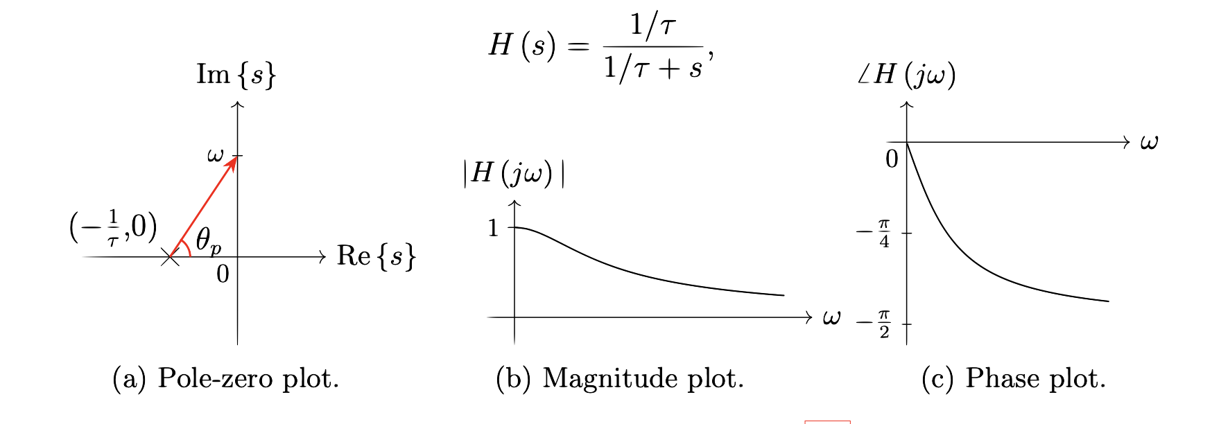
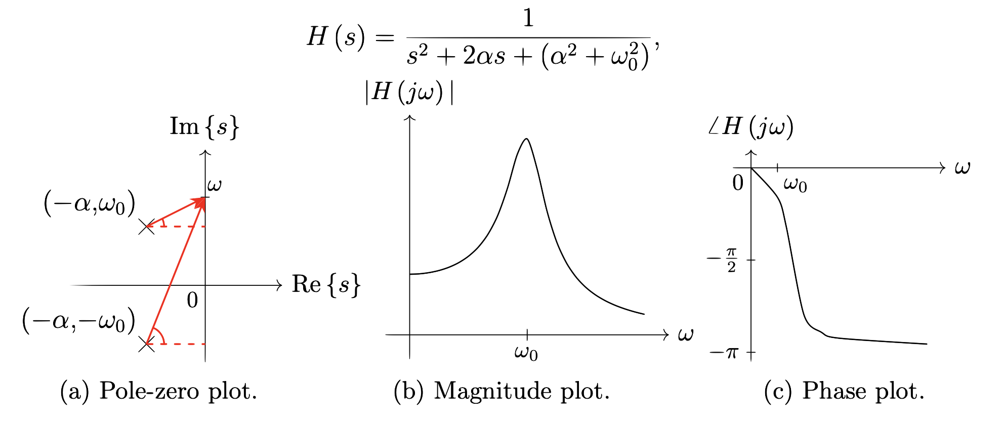
Figure 5.1.b. Basic analog LPF: a single real pole at \(s=-1/\tau\) sets \(\Omega_c=1/\tau\); \(|H(j\Omega)|\) decays smoothly, \(\angle H(j\Omega)\) from \(0\) toward \(-\pi/2\).Figure 5.1.c. Basic analog BPF: a conjugate pole pair at \((-\alpha,\pm\Omega_0)\) — the RLC resonance of Example 2.7, read as a filter; \(|H(j\Omega)|\) peaks at \(\omega_0\).
An all-pass filter (APF) has unity magnitude at every frequency but changes phase. It does not alter the amplitude spectrum, yet it can change the timing and shape of a waveform:
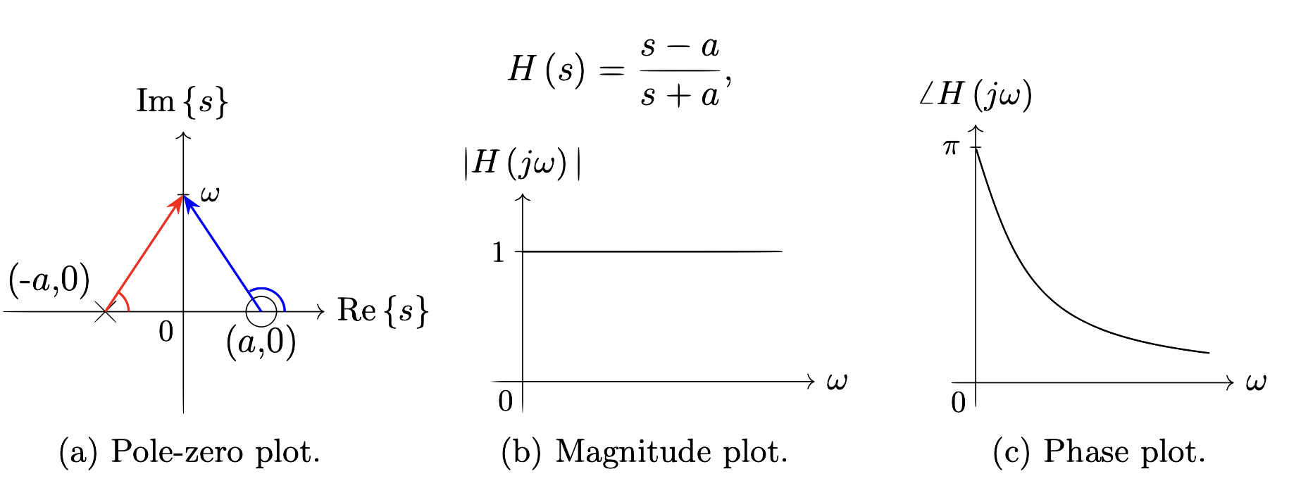
The pole at \(s=-a\) and zero at \(s=+a\) are mirror images across the \(j\Omega\)-axis. Their distances to \(j\Omega\) are equal, so their magnitude effects cancel. Their angles are different, so a frequency-dependent phase shift remains. Cascading an all-pass section with another filter can therefore adjust phase without changing the designed magnitude response.
Figure 5.1.d. The all-pass filter \(H(s)=(s-a)/(s+a)\): a pole and zero mirrored across the \(j\Omega\)-axis, so their magnitude vectors are always equal — \(|H(j\Omega)|=1\) for every \(\Omega\), while the phase runs from \(\pi\) at \(\Omega=0\) down toward \(0\), the one filter type in this catalogue defined entirely by what it does to phase, useful precisely because Section 6.3 shows no IIR filter's phase is under the designer's direct control otherwise.
5.2 The ideal filter cannot be built
Take the ideal low-pass of Figure 5.1.a literally, \(H_i(j\Omega)=\mathrm{rect}(\Omega/2\Omega_c)\), and invert it with the CTFT pair of Section 2.9.1 (duality: a rectangle in frequency is a sinc in time):
The ideal impulse response is both non-causal, because it is non-zero before the input arrives, and infinite in duration. A physical circuit cannot implement either property exactly.
Step
What it costs
1. Make it causal \(h_1(t)=h_i(t)u(t)\)
Throws away the \(t<0\) half, losing 50% of the energy and, with it, the ideal shape.
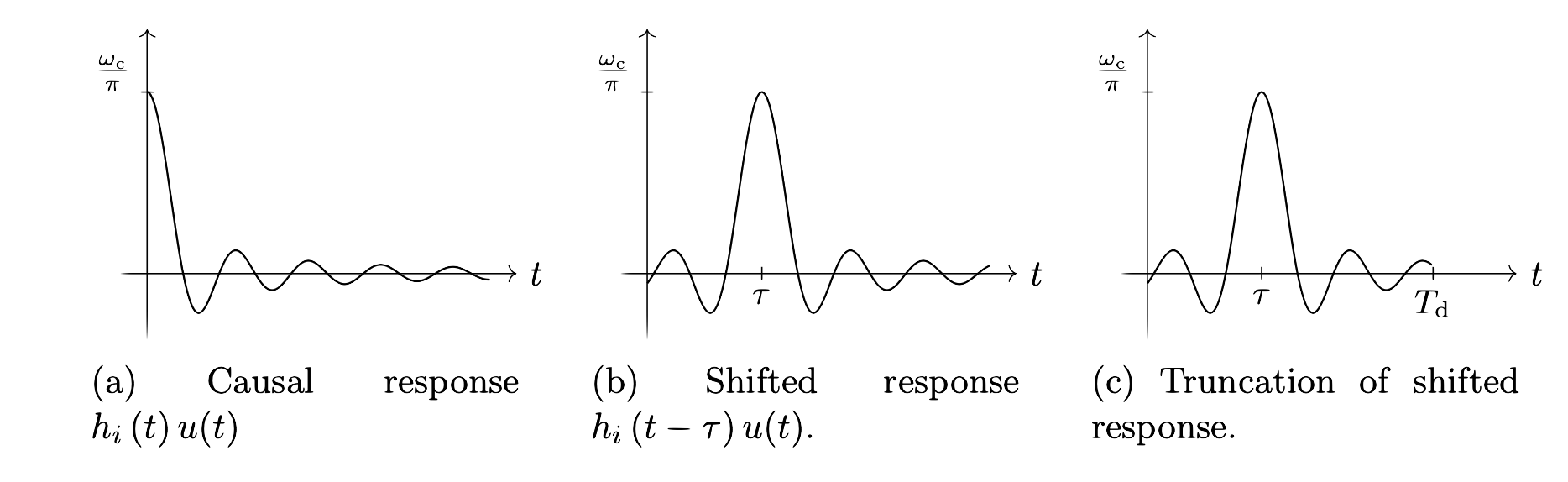
2. Delay it \(h_2(t)=h_i(t-\tau)u(t)\)
A pure delay only adds linear phase (Eq. 2.22); it does not touch \(|H(j\Omega)|\), so shifting first and truncating second keeps more of the response.
3. Truncate \(h_3=h_2\cdot u(T_d-t)\)
Now finite and causal — but a hard cut is a rectangular window (Section 2.9.3), and windowing convolves the ideal spectrum with a sinc: ripple (Gibbs) appears at the corner.
4. Taper \(h_{\text{prac}}=h_2\cdot w(t)\)
A smooth window \(w(t)\) trades main-lobe width for lower ripple — the same rectangular-vs-tapered trade Section 2.9.3 already made for the DFT.
Figure 5.2. Steps 1–3 made visible: (a) truncating \(h_i(t)\) to \(t\ge0\) throws away its symmetric left half; (b) delaying by \(\tau\) restores that lost half without touching \(|H(j\Omega)|\) — only the peak moves, to \(t=\tau\); (c) truncating at \(t=T_d\) finally makes it finite, ready for Step 4's windowing.
Classical analog design does not build \(h(t)\) directly at all; it works backwards from a target magnitude shape that a real RLC network (or an active op-amp circuit) can realise exactly, which is the subject of the rest of this lecture.
5.3 The design framework: one prototype, four filters
Every classical analog design, whatever the target shape, follows the same five moves:
1 · Normalize
Passband/stopband edges and gains become the dimensionless numbers \((A_p,\Omega_p,A_s,\Omega_s)\).
2 · Design LPP
Build a low-pass prototype at \(\Omega_c=1\,\text{rad/s}\) — Sections 5.4, 5.6, 5.7.
3 · Transform
Apply \(s\mapsto F(s)\) to turn the LPP into an HPF, BPF or BSF (Section 5.5).
4 · Denormalize
Scale the normalized cutoff up to the real \(\Omega_c\).
5 · Optional
Bilinear-transform \(s\to z\) for a digital filter — Lecture 6.
Why bother with a prototype at all
The main design choice is the low-pass prototype: its family and order determine ripple, transition sharpness and complexity. Standard frequency transformations then convert that prototype into a high-pass, band-pass or band-stop filter.
5.3.1 A first look at the four classical families
Sections 5.4, 5.6 and 5.7 derive three of these families in full; naming all four now, side by side, gives every derivation that follows a place to land.
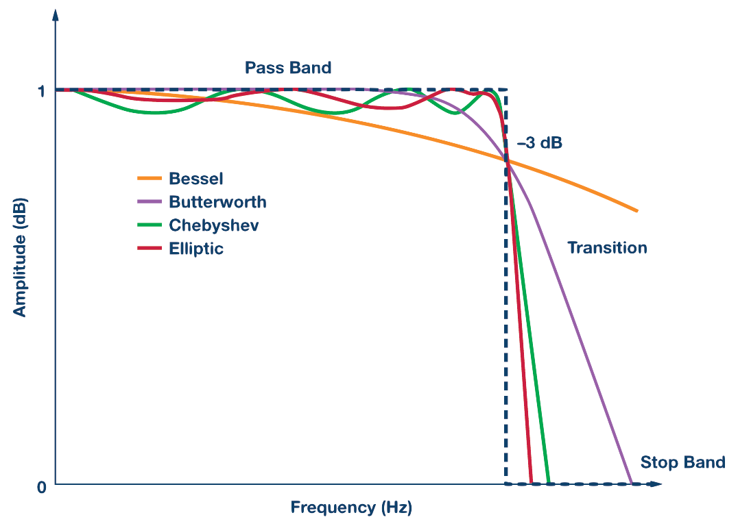
Figure 5.3.a. The four families on one low-pass specification: Bessel's gentlest roll-off (no ripple, best phase), Butterworth's monotonic curve, Chebyshev's passband ripple, and elliptic's sharpest transition — all meeting the same \(-3\,\text{dB}\) point, at very different cost.
Family
Passband
Stopband / transition
Phase & order
Bessel
Monotonic, no ripple
Gentlest roll-off of the four
Best linear phase; highest order for a given cutoff sharpness
Butterworth
Monotonic, maximally flat (Eq. 5.4)
Smooth, moderate roll-off
Moderate phase distortion; moderate order
Chebyshev I/II
Equiripple (I) or flat (II)
Sharper than Butterworth for the same order
Worse phase than Butterworth; fewer poles for the same spec
Elliptic
Equiripple (Eq. 5.13)
Sharpest of the four
Worst phase linearity; lowest order of all four
5.3.2 The vocabulary every specification is written in
Whatever the family, a specification is always drawn as three regions of \(|H(j\Omega)|\) separated by two frequencies:
Passband
\(\Omega<\Omega_p\): gain must stay at or above \(A_p\) — the signal must pass through.
Transition band
\(\Omega_p<\Omega<\Omega_s\): no constraint is placed here — the filter is free to roll off however it can.
Stopband
\(\Omega>\Omega_s\): gain must stay at or below \(A_s\) — the signal must be rejected.
Figure 5.3.b. The three regions every specification divides \(|H(j\Omega)|\) into: a guaranteed passband below \(\Omega_p\), a free transition band, and a guaranteed stopband above \(\Omega_s\). Eq. (5.5)–(5.6) and their Chebyshev/elliptic counterparts are exactly the algebra that finds the smallest filter satisfying these four numbers, \((A_p,\Omega_p,A_s,\Omega_s)\).
5.4 The Butterworth prototype: maximally flat
Butterworth's defining property is a magnitude-squared that is as flat as a rational function of order \(N\) can possibly be at \(\Omega=0\) — no ripple, only a smooth monotonic roll-off:
A Butterworth design must determine two quantities: the order \(N\) and the cutoff \(\Omega_c\). The specification gives a minimum allowed gain \(A_p\) at the passband edge \(\Omega_p\) and a maximum allowed gain \(A_s\) at the stopband edge \(\Omega_s\). Applying Eq. (5.4) at both edges gives the required order:
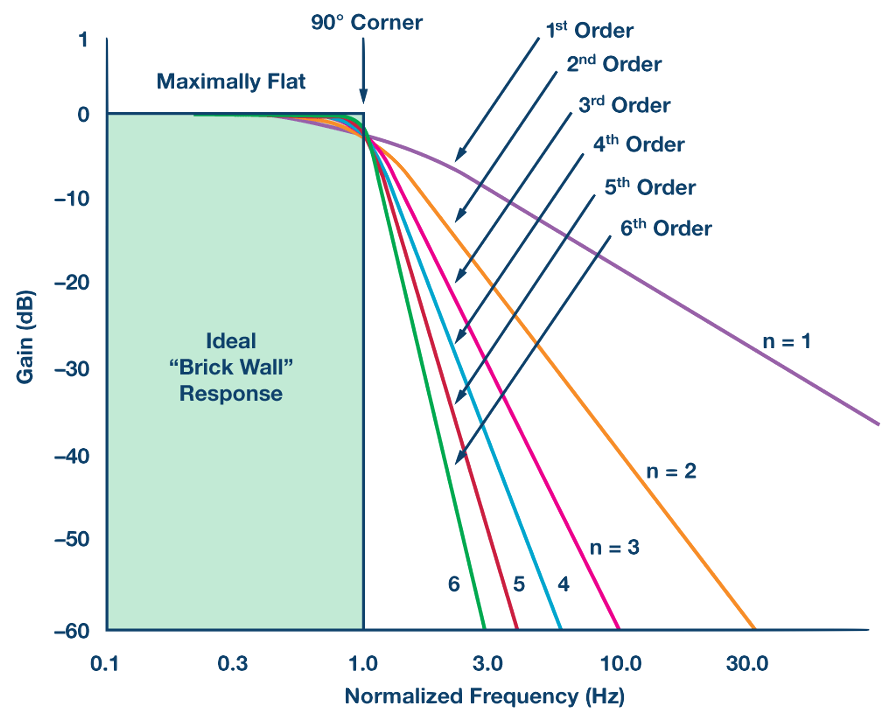
A Butterworth response approaches the ideal low-pass shape as the order increases. Each additional pole makes the transition steeper, but also increases circuit complexity and sensitivity.
Figure 5.4.a. As \(N\) grows from 1st to 6th order, the Butterworth curve hugs the \(90^\circ\) corner more and more tightly, converging on the ideal brick wall in the limit \(N\to\infty\) — but every extra order in Eq. (5.4) is another pole, i.e. another reactive component and another degree of design and tuning complexity in the real circuit. Sharper is never free; it is only ever purchased with hardware.
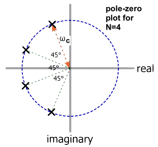
For a normalized prototype with \(\Omega_c=1\), the poles are equally spaced on the unit circle. Only the left-half-plane poles are used, because they have negative real parts and therefore produce a stable causal filter:
Figure 5.4.b. For \(N=4\), Eq. (5.7) places four poles on the circle of radius \(\Omega_c=1\) (the LPF prototype's normalized cutoff), each separated from its neighbour by exactly \(180^\circ/N=45^\circ\) — only the left half is kept, since the right-half poles that complete the uniform spacing would be unstable (Eq. 4.8). No pole sits closer to the \(j\Omega\)-axis than any other; that uniform angular spacing is precisely what “maximally flat” means geometrically, and it is why no single frequency near \(\Omega_c\) gets singled out for a resonant peak the way Section 6.5's two-pole resonator deliberately creates one.
EXAMPLE 5.1 · Designing a Butterworth low-pass filter
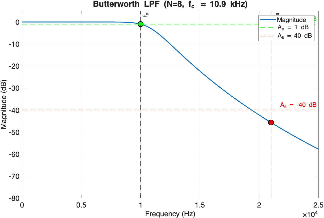
An analog LPF must satisfy \(f_p=10\,\text{kHz}\), \(f_s=21\,\text{kHz}\), \(G_p=-1\,\text{dB}\), \(G_s=-40\,\text{dB}\). Find \(N\), \(\Omega_c\), and \(H(s)\).
Step 1 · Linear gains and edges. \(A_p=10^{-1/20}\approx0.8913\), \(A_s=10^{-40/20}=0.01\), \(\Omega_p=2\pi f_p\), \(\Omega_s/\Omega_p=f_s/f_p=2.1\).
Step 2 · Order. By Eq. (5.5): \(1/A_p^2-1\approx0.259\), \(1/A_s^2-1=9999\), so \((\Omega_s/\Omega_p)^{2N}\approx3.86\times10^4\) and
Step 3 · Cutoff. By Eq. (5.6) with \(N=8\): \((0.259)^{-1/16}\approx1.088\), so \(\Omega_c\approx\Omega_p\cdot1.088\approx6.84\times10^4\,\text{rad/s}\) (\(f_c\approx10.9\,\text{kHz}\)).
Step 4 · Check. \(|H(j\Omega_p)|=1/\sqrt{1+0.259}=0.8913=A_p\ \checkmark\), and \(|H(j\Omega_s)|\approx0.0051\le A_s=0.01\ \checkmark\) (with margin, since \(N\) was rounded up).
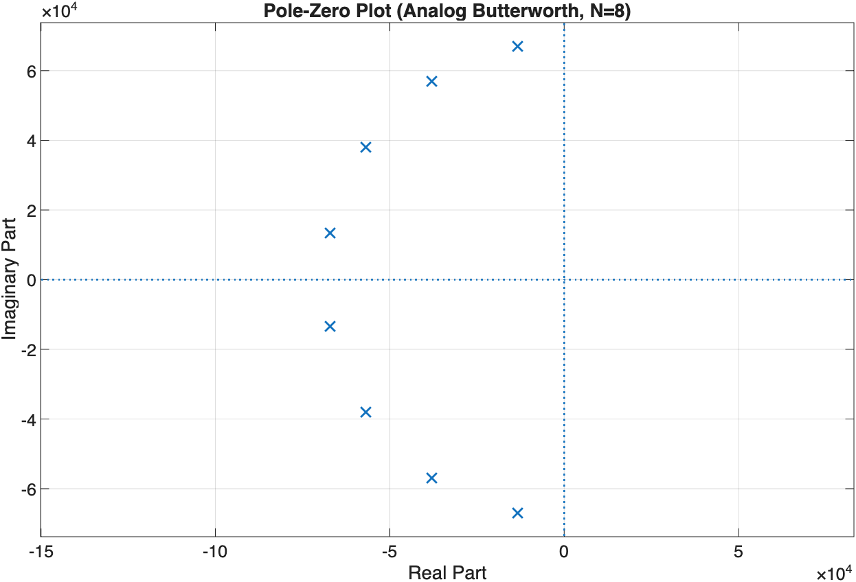
Eight poles, equally spaced on a circle of radius \(6.84\times10^4\,\text{rad/s}\) (Eq. 5.7), give \(H(s)=K/\prod_{k=1}^{8}(s-p_k)\) with \(K\) fixed by unity DC gain. The rounding in Step 2 is why the stopband check has margin to spare: real designs almost never land exactly on the boundary.
MATLAB Corner for Example 5.1
This script reproduces Example 5.1 from scratch, computing \(N\) and \(\Omega_c\) by hand-coding Eqs. (5.5)–(5.6), then builds \(H(s)\) with butter and evaluates \(H(j\Omega)\) manually via polyval — the same Eq. (5.2) split into magnitude and phase, done numerically.
Goal: compute \(N\) and \(\Omega_c\) for Example 5.1's specification (Eqs. 5.5-5.6), then plot the magnitude with the spec points \(f_p,f_s\) marked and simulated exactly, plus the resulting pole-zero layout in the \(s\)-plane.
Figure 5.4.c.Checking the Butterworth design in MATLAB. The green marker at the passband edge \(f_p\) remains above the \(-1\,\text{dB}\) limit, while the red marker at \(f_s\) lies below the required \(-40\,\text{dB}\) stopband level. The curve decreases smoothly without ripple, which is the defining Butterworth behaviour. The pole–zero plot gives a second check: all eight poles lie on the circle \(|s|=\Omega_c\approx6.84\times10^4\,\text{rad/s}\), and only the left-half-plane roots are used. Their negative real parts make the realised filter stable.
5.5 Frequency transformations: one prototype, four filters
A normalized low-pass prototype can be converted into a high-pass, band-pass or band-stop filter by replacing \(s\) with a standard function of \(s\). For band filters, \(\Omega_0=\sqrt{\Omega_1\Omega_2}\) is the centre frequency and \(B=\Omega_2-\Omega_1\) is the bandwidth:
Target
Substitute \(s\to\) …
HPF
\(\Omega_c/s\) — same order, same \(\Omega_c\), \(N\) zeros appear at \(s=0\).
BPF
\((s^2+\Omega_0^2)/(Bs)\) — order doubles to \(2N\); each LPF pole becomes a conjugate pair.
BSF
\(Bs/(s^2+\Omega_0^2)\) — order doubles; zeros land exactly at \(\pm j\Omega_0\), a deep notch.
Apply the HPF mapping to Example 5.1's \(H_{LP}(s)=K/\prod_{k=1}^{8}(s-p_k)\) and multiply through by \(s^8\):
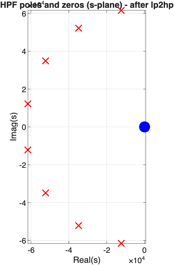
For the low-pass-to-high-pass transformation, each prototype pole \(p_k\) maps to \(\Omega_c^2/p_k\). A stable left-half-plane pole remains in the left half-plane, so the transformation preserves stability.
EXAMPLE 5.2 · Turning Example 5.1's LPF into a highpass
Continuing Example 5.1's spec (\(f_p=10\,\text{kHz}\), \(f_s=21\,\text{kHz}\), \(G_p=-1\,\text{dB}\), \(G_s=-40\,\text{dB}\)), design the analog highpass counterpart: find its order and cutoff, and verify where its zeros land.
Step 1 · Order is unchanged. Eq. (5.5)'s order formula depends only on the ratio \(\Omega_s/\Omega_p\) (through its square, via \(\ln^2\)), and inverting a highpass's edges to their lowpass-equivalent reciprocals leaves that ratio's magnitude unchanged: \(|\ln(\Omega_p/\Omega_s)|=|\ln(\Omega_s/\Omega_p)|\). So the highpass needs exactly the same order as Example 5.1: \(\boxed{N=8.}\)
Step 2 · Cutoff. Take the passband edge itself as the highpass cutoff, \(\Omega_c=\Omega_p=2\pi(10\,\text{kHz})\approx6.28\times10^4\,\text{rad/s}\) — everything above this frequency must clear \(A_p\), exactly the boundary condition Eq. (5.4) enforces at \(\Omega=\Omega_c\).
Step 3 · Transform the poles. By Eq. (5.8), each LPF pole \(p_k\) maps to \(\Omega_c^2/p_k\), and the transfer function picks up \(N=8\) zeros at \(s=0\) (from multiplying through by \(s^8\)) — the DC block that turns a low-pass into a high-pass.
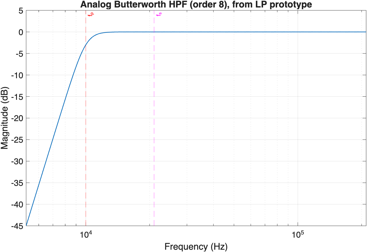
Step 4 · What MATLAB confirms.buttord returns the same \(N=8\) (the reciprocal-ratio symmetry of Step 1, verified numerically); lp2hp's returned numerator has degree \(8\) with all eight roots at the origin, and the resulting magnitude plot passes cleanly above \(f_p\) and is buried in the stopband well before \(f_s\) — the MATLAB corner below is exactly this check.
MATLAB Corner for Example 5.2
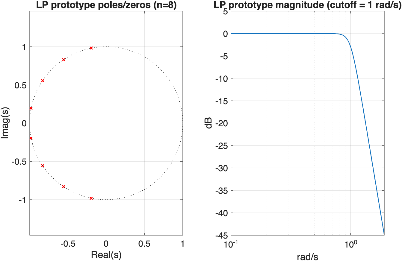
Goal: transform a Butterworth LPF prototype into an analog HPF via lp2hp, and confirm the zeros land at \(s=0\) exactly as Eq. (5.8) predicts.
Butterworth_HPF.m
MATLAB
%% Butterworth_HPF.m - LP prototype transformed to an analog HPF (Eq. 5.8)
title('HPF poles and zeros (s-plane) - after lp2hp', 'FontSize',16);
set(gca, 'FontSize',12);
axis tight; % or set specific limits, e.g., axis([-wp wp -wp wp]);
drawnow;
Figure 5.5.a.What changes in the low-pass-to-high-pass transformation. MATLAB first designs the low-pass prototype and then applies lp2hp. The transformation moves each prototype pole from \(p_k\) to \(\Omega_c^2/p_k\), in agreement with Eq. (5.8). It also places \(n\) zeros at \(s=0\). Those zeros force the gain to zero at DC, which is exactly what a high-pass filter requires. The transformed magnitude is small below the cutoff and approaches its passband level at high frequency.
EXAMPLE 5.3 · Designing a band-pass from scratch
Design a Butterworth BPF with passband \(15\text{-}20\,\text{kHz}\), stopband edges \(12\,\text{kHz}\) and \(25\,\text{kHz}\), \(A_p=1\,\text{dB}\), \(A_s=40\,\text{dB}\). Find the order, centre frequency and bandwidth.
Step 1 · Centre and bandwidth. \(\Omega_0=\sqrt{\Omega_{p1}\Omega_{p2}}=\sqrt{15\times20}\,\text{kHz}\approx17.32\,\text{kHz}\), \(B=\Omega_{p2}-\Omega_{p1}=5\,\text{kHz}\).
Step 2 · Map each edge to an equivalent LPF frequency. The bandpass-to-lowpass frequency warp is \(\Omega_{\text{eq}}=|\Omega^2-\Omega_0^2|/(\Omega B)\). At both passband edges this equals exactly \(1\) by construction (\(|15^2-300|/(15\times5)=75/75=1\); \(|20^2-300|/(20\times5)=100/100=1\)) — confirming \(\Omega_{p,\text{eq}}=1\), the LPP's own cutoff. At the stopband edges: \(|12^2-300|/(12\times5)=156/60=2.6\) and \(|25^2-300|/(25\times5)=325/125=2.6\) — both edges give the same equivalent stopband frequency, \(\Omega_{s,\text{eq}}=2.6\), a geometrically symmetric specification.
Step 3 · Order. This is now a plain Eq. (5.5) LPF problem with \(\Omega_s/\Omega_p=2.6\):
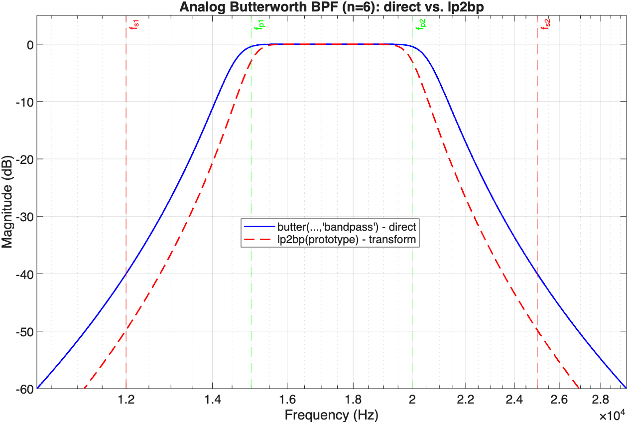
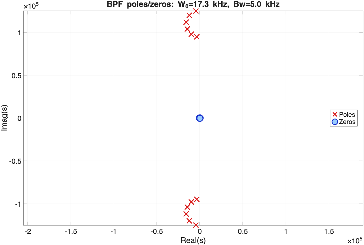
Step 4 · What MATLAB confirms.buttord(Wp,Ws,Ap,As,'s') performs exactly this frequency-warp internally and returns the same \(N=6\) (visible in the MATLAB corner's magnitude-plot title below); the pole–zero plot's poles straddling \(\Omega_0=17.3\,\text{kHz}\) confirm Step 1's centre frequency directly.
MATLAB Corner for Example 5.3
Goal: build an analog BPF two ways — directly with butter(...,'bandpass') and via lp2bp from a LP prototype — and confirm they agree, then read the doubled pole count off the pole-zero plot.
Butterworth_BPF.m
MATLAB
%% Butterworth_BPF.m - LP prototype transformed to an analog BPF (Eq. 5.8-kin)
Figure 5.5.b.Checking the band-pass transformation. The direct butter result and the transformed lp2bp result lie on top of each other, showing that the two design routes produce the same transfer function. A low-pass filter of order \(n\) becomes a band-pass filter of order \(2n\): every prototype pole produces a pair of poles around the centre frequency. The response is largest between the two passband edges and decreases on both sides, while the pole–zero map confirms the expected doubled order.
EXAMPLE 5.4 · An asymmetric band-stop, and why both edges must be checked
Design a Butterworth BSF with passband edges \(15\,\text{kHz}\) and \(27\,\text{kHz}\), stopband edges \(10\,\text{kHz}\) and \(32\,\text{kHz}\), \(A_p=1\,\text{dB}\), \(A_s=40\,\text{dB}\). Find the order.
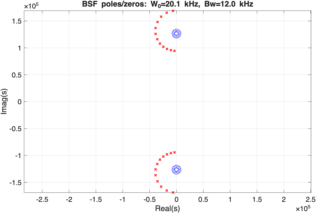
Step 1 · Centre and bandwidth. \(\Omega_0=\sqrt{15\times27}\,\text{kHz}=\sqrt{405}\approx20.12\,\text{kHz}\), \(B=27-15=12\,\text{kHz}\) — exactly what the MATLAB corner's pole-zero title reports.
Step 2 · Map both stopband edges — this spec is not symmetric. Unlike Example 5.4, \(10\,\text{kHz}\) and \(32\,\text{kHz}\) are not equally spaced from \(\Omega_0\) on a log scale, so the two edges give different equivalent lowpass frequencies: at \(10\,\text{kHz}\), \(|10^2-405|/(10\times12)=305/120\approx2.54\); at \(32\,\text{kHz}\), \(|32^2-405|/(32\times12)=619/384\approx1.61\).
Step 3 · The tighter edge wins. A smaller equivalent-frequency ratio means less separation between pass and stop in the equivalent LPF, so it demands the higher order. \(1.61<2.54\), so \(32\,\text{kHz}\) is the binding constraint:
Step 4 · The lesson. Had the design only checked the \(10\,\text{kHz}\) edge, it would have wrongly concluded \(N=6\) suffices — half the true order — and shipped a filter that fails its spec above \(27\,\text{kHz}\). buttord checks both edges automatically and returns the safe \(N=12\); this is exactly why Eq. (5.5) must be applied to every stopband edge in an asymmetric specification, not just the nearer-looking one.
MATLAB Corner for Example 5.4
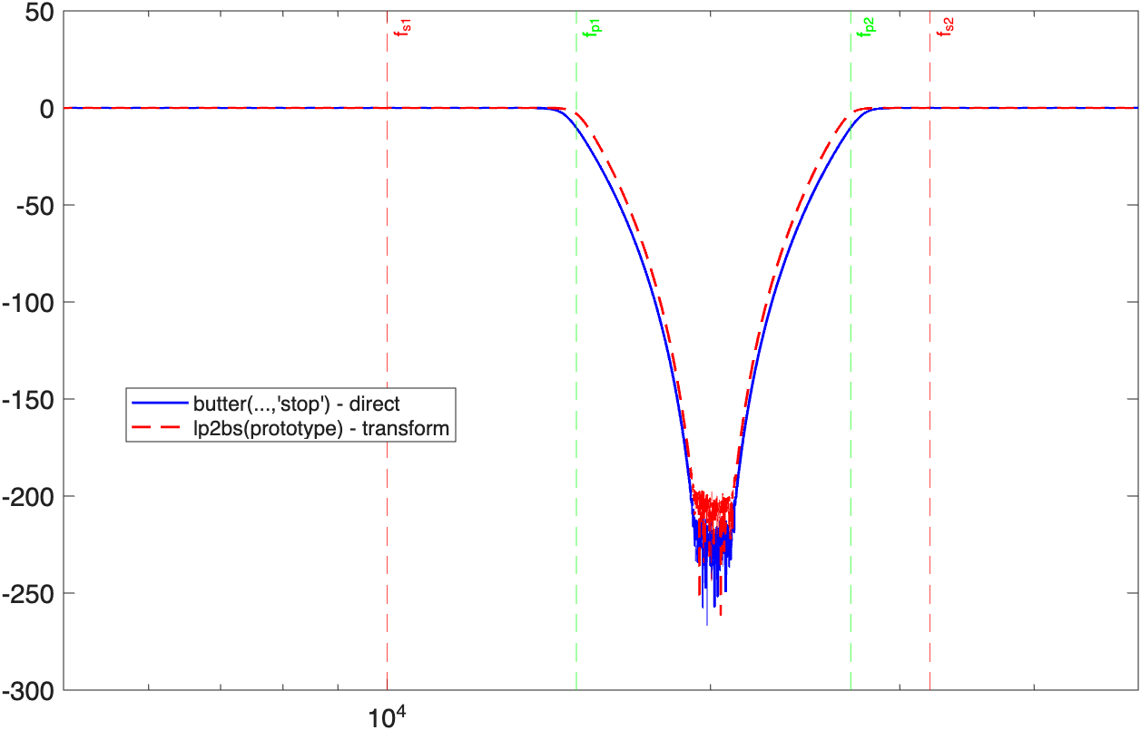
Goal: build the band-stop counterpart with lp2bs, and confirm its zeros land exactly at \(\pm j\Omega_0\) — the deep notch Section 5.5 promised.
Butterworth_BSF.m
MATLAB
%% Butterworth_BSF.m - LP prototype transformed to an analog BSF
Figure 5.5.c.Checking the band-stop transformation. The direct design and the transformed prototype give almost identical magnitude curves. Their small difference at the bottom of the notch is numerical round-off: both theoretical responses are zero there. The pole–zero map explains the notch. Zeros at \(s=\pm j\Omega_0\) place a zero directly on the frequency axis at the centre frequency, forcing \(|H(j\Omega_0)|=0\). The surrounding poles set the width and shape of the rejected band.
5.6 Chebyshev prototypes: trading flatness for a sharper corner
Butterworth filters use their degrees of freedom to keep the passband smooth and monotonic. Chebyshev filters allow an equiripple error that moves between fixed limits. Accepting this ripple gives a steeper transition for the same order, or a lower order for the same specification.
The Chebyshev polynomial \(C_N\) oscillates between bounded values for \(|x|\le1\), which creates the passband ripple, and grows rapidly for \(|x|>1\), which creates the sharp stopband roll-off. The passband requirement determines the ripple factor \(\varepsilon\), and the stopband requirement determines the order:
The prototype poles (\(\Omega_p=1\)) sit on an ellipse, not a circle — the price of ripple is that the equal-spacing symmetry of Figure 5.4.b is broken deliberately, trading it for a sharper knee:
Swap which band absorbs the ripple and you get Type II: a monotonic, flat passband (no ripple where you are most likely to care) and equiripple in the stopband instead, with the roles of \(\Omega_p\) and \(\Omega_s\) exchanged inside \(C_N\):
Both types need the same order \(N\) for the same specification — the polynomial doing the work is identical, only which band it ripples in differs — so the choice between them is purely about which band you can tolerate ripple in, never about cost.
EXAMPLE 5.5 · The same specification, a Chebyshev Type I filter
Design a Chebyshev Type I LPF for Example 5.1's exact specification (\(f_p=10\,\text{kHz}\), \(f_s=21\,\text{kHz}\), \(G_p=-1\,\text{dB}\), \(G_s=-40\,\text{dB}\)), and compare the order to Butterworth's.
Step 1 · Ripple factor. By Eq. (5.10), \(\varepsilon=\sqrt{A_p^{-2}-1}=\sqrt{1.259-1}\approx0.509\), fixed by the passband spec alone.
Step 2 · Order. With \(k_s=\Omega_s/\Omega_p=2.1\): \(\mathrm{arccosh}(2.1)\approx1.37\), and \(\sqrt{A_s^{-2}-1}/\varepsilon\approx99.995/0.509\approx196.5\), \(\mathrm{arccosh}(196.5)\approx5.97\), so
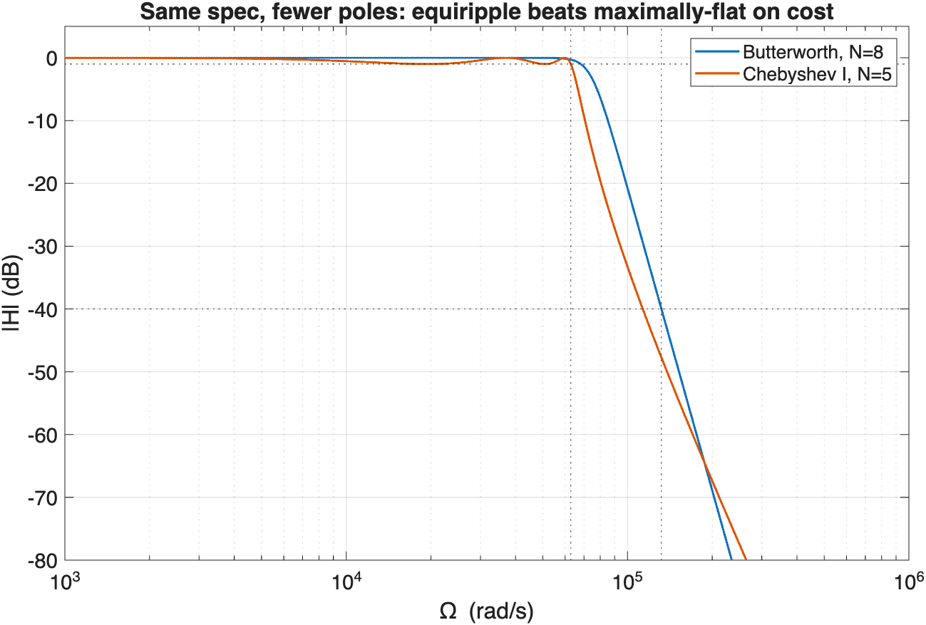
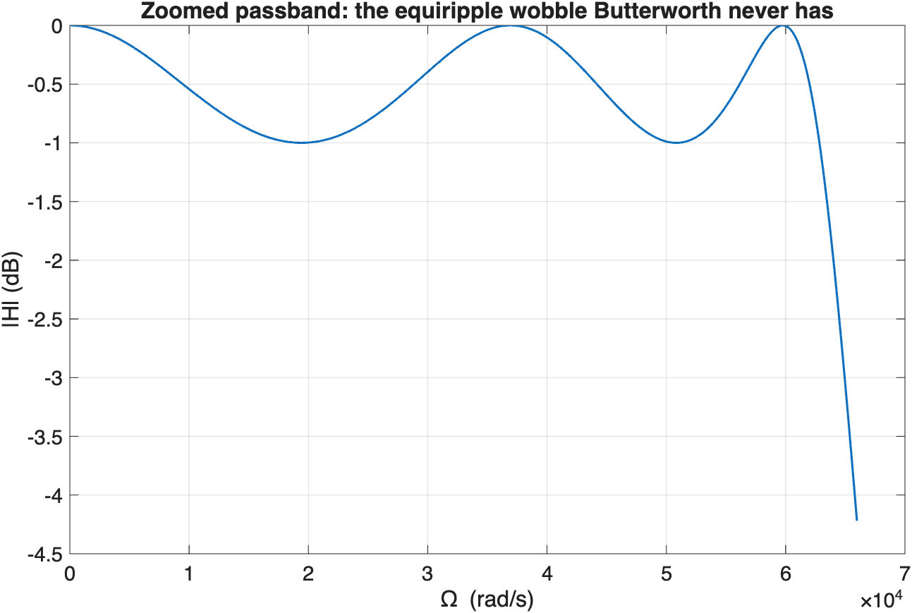
Step 3 · The payoff. Five poles instead of Butterworth's eight for the identical spec — equiripple flatness buys almost 40% fewer components for the same passband/stopband guarantee. The cost is a passband that wobbles between \(A_p\) and \(1\) instead of decaying smoothly, and a pole placement (Eq. 5.11, an ellipse) that is more sensitive to component tolerances than Butterworth's circle.
MATLAB Corner for Example 5.5
This script builds Example 5.5's Chebyshev Type I filter with cheb1ord/cheby1 and overlays it on Example 5.1's Butterworth, on the same axes, so the order saving and the ripple trade-off are visible in one picture.
Goal: confirm Chebyshev Type I needs \(N=5\) against Butterworth's \(N=8\) for the identical spec, and see the equiripple passband directly.
chebyshev_vs_butterworth.m
MATLAB
%% chebyshev_vs_butterworth.m - same spec, two families (Eq. 5.10 vs Eq. 5.5)
title('Zoomed passband: the equiripple wobble Butterworth never has');
xlabel('\Omega (rad/s)'); ylabel('|H| (dB)');
Figure 5.6.Butterworth and Chebyshev Type I compared. Both filters satisfy the same passband and stopband limits, but they use the allowed error differently. The Butterworth response is smooth and monotonic, so it needs the higher order. The Chebyshev Type I response deliberately ripples within the permitted passband. In return, it changes more rapidly through the transition region and reaches the stopband requirement with three fewer poles. The zoomed passband makes the price of that lower order visible.
5.7 Elliptic (Cauer) filters: equiripple in both bands
Push the same idea one step further: ripple in both bands at once, and the transition gets as sharp as a given order can possibly make it.
Elliptic filters allow ripple in both the passband and stopband. For a fixed specification, they usually achieve the lowest order of the classical families studied here. Their finite zeros on the \(j\Omega\)-axis create deep stopband nulls and a very sharp transition. The costs are a more complicated pole–zero pattern, greater sensitivity, and typically the least linear phase.
5.8 Choosing a prototype
Choosing a family means deciding where ripple is acceptable and how much filter order can be afforded. A further family, Bessel, is not derived here but is useful when waveform shape and nearly linear phase matter more than a sharp transition.
Butterworth
Chebyshev I / II
Elliptic
Order for fixed spec
Flat pass, no ripple
Ripple in pass (I) or stop (II)
Ripple in both
Highest → lowest, left to right
Poles on a circle
Poles on an ellipse
Poles+zeros, most complex
Phase linearity: best → worst, left to right
Use Butterworth for a smooth response, Chebyshev when a sharper transition is worth allowing ripple in one band, and elliptic when the narrowest transition and lowest order are the main priorities. MATLAB provides butter, cheby1, cheby2 and ellip, but the specification and trade-off still need to be understood before selecting a family.
EXAMPLE 5.6 · All four families, one spec, one table
For Example 5.1's exact specification, state (deriving where this lecture has given you the tools to, and citing MATLAB otherwise) the minimal order of all four classical families.
Butterworth: \(N=8\). Exactly Example 5.1's Eq. (5.5) calculation — nothing new to derive.
Chebyshev I: \(N=5\). Exactly Example 5.5's Eq. (5.10) calculation.
Chebyshev II: \(N=5\). Section 5.6.2 established that Type II needs the identical order to Type I for the same spec — the underlying polynomial \(C_N\) is the same, only which band it ripples in differs. No new calculation needed.
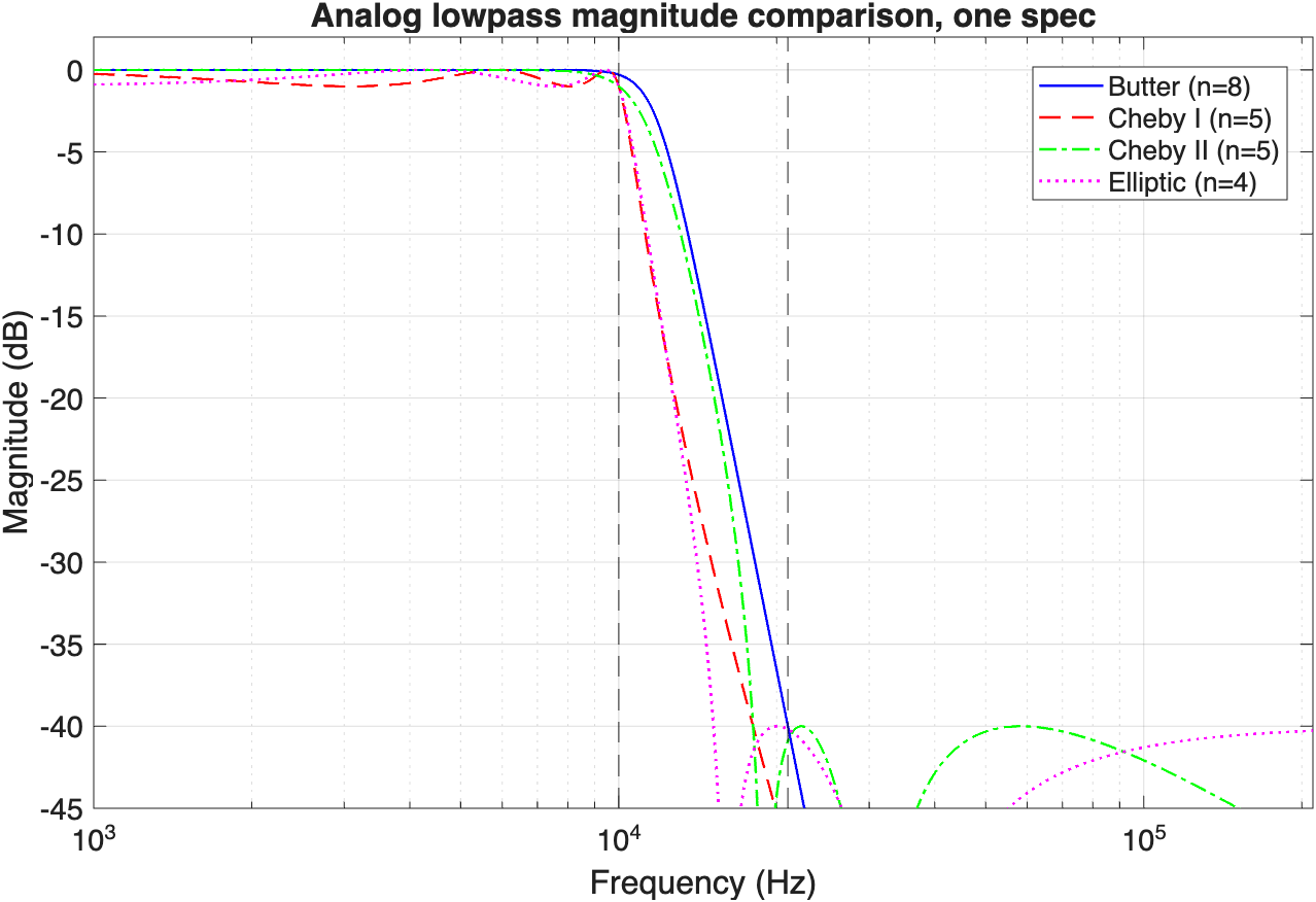
Elliptic: \(N=4\), cited from ellipord. Section 5.7 deliberately stopped short of deriving Eq. (5.13)'s order formula by hand: it requires the Jacobi elliptic rational function \(R_N(\xi,\cdot)\) and elliptic integrals, well beyond this module's scope. What Section 5.7 promised — the lowest order of the four families — is confirmed here numerically: \(4<5\le5<8\), exactly the ranking Section 5.8's comparison table names, with the exact numbers this time rather than just the ordering.
MATLAB Corner for Example 5.6
This script puts all four families head to head on the identical specification, computing each one's minimal order with its own *ord function and overlaying the results — the single clearest picture of Section 5.8's trade-off.
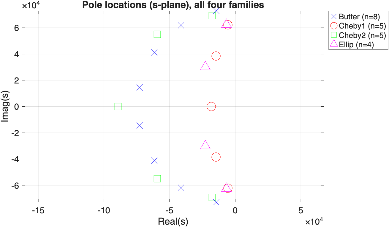
Goal: confirm the order ranking Butterworth > Chebyshev > elliptic for one fixed spec, and see all four pole layouts on one (s)-plane axis.
compare_analog.m
MATLAB
%% compare_analog.m - Butterworth vs Chebyshev I/II vs Elliptic, one spec
fp = 10e3; fs = 21e3; Ap = 1; As = 40;
Wp = 2*pi*fp; Ws = 2*pi*fs;
[n_b,Wb] = buttord(Wp,Ws,Ap,As,'s');
[n_c1,Wc1] = cheb1ord(Wp,Ws,Ap,As,'s');
[n_c2,Wc2] = cheb2ord(Wp,Ws,Ap,As,'s');
[n_e,We] = ellipord(Wp,Ws,Ap,As,'s');
[z_b,p_b,k_b] = butter(n_b, Wb, 's');
[z_c1,p_c1,k_c1] = cheby1(n_c1, Ap, Wc1, 's');
[z_c2,p_c2,k_c2] = cheby2(n_c2, As, Wc2, 's');
[z_e,p_e,k_e] = ellip(n_e, Ap, As, We, 's');
[num_b,den_b] = zp2tf(z_b,p_b,k_b);
[num_c1,den_c1] = zp2tf(z_c1,p_c1,k_c1);
[num_c2,den_c2] = zp2tf(z_c2,p_c2,k_c2);
[num_e,den_e] = zp2tf(z_e,p_e,k_e);
w = logspace(log10(Wp)-1, log10(Ws)+1, 8192); f = w/(2*pi);
figure('Color','w');
semilogx(f, 20*log10(abs(freqs(num_b,den_b,w))), 'b-', 'LineWidth',1.2); hold on;
Figure 5.8.Comparing all four analog families. MATLAB applies the same specification to each family. Butterworth needs the highest order because it allows no ripple. Chebyshev Types I and II reduce the order by allowing ripple in one band. The elliptic design allows ripple in both bands and reaches the specification with the lowest order. The pole–zero plots show the different mechanisms: poles closer to the \(j\Omega\)-axis create sharper changes, and the finite transmission zeros of Chebyshev II and elliptic filters deepen the stopband. The gain is efficiency; the usual cost is a less linear phase and a more sensitive design.
?Problems with solutions
Work each one before reading the solution.
PROBLEM 5.1
A Butterworth LPF must satisfy \(f_p=1\,\text{kHz}\), \(f_s=3\,\text{kHz}\), \(G_p=-3\,\text{dB}\), \(G_s=-30\,\text{dB}\). Find \(N\) and \(\Omega_c\).
Solution. \(A_p=10^{-3/20}\approx0.7079\), \(A_s=10^{-30/20}\approx0.0316\), \(\Omega_s/\Omega_p=f_s/f_p=3\). Since \(G_p=-3\,\text{dB}\) is exactly the Butterworth \(-3\,\text{dB}\) point, \(1/A_p^2-1=1\) exactly.
And since \(1/A_p^2-1=1\) exactly, Eq. (5.6) collapses to \(\Omega_c=\Omega_p\cdot1^{-1/(2N)}=\Omega_p=2\pi(1000)\approx6283\,\text{rad/s}\): whenever the passband spec is the \(-3\,\text{dB}\) point, \(\Omega_c=\Omega_p\) with no computation at all.
PROBLEM 5.2
A normalized Butterworth LPF (\(N=3\), \(\Omega_c=1\)) must become a band-pass filter with centre \(\Omega_0=1000\,\text{rad/s}\) and bandwidth \(B=200\,\text{rad/s}\). What is the resulting filter's order, and what mapping produces it?
Solution. The BPF mapping of Table in Section 5.5 is \(s\to(s^2+\Omega_0^2)/(Bs)=(s^2+10^6)/(200s)\). Substituting into \(H_{LP}(s)=K/\prod_{k=1}^{3}(s-\bar p_k)\) turns each of the 3 linear factors into a quadratic in \(s\) (Eq. 5.8's BPF cousin), so the denominator degree doubles:
$$\boxed{\text{order}=2N=6.}$$
Each of the original 3 real-axis-relative poles becomes a complex-conjugate pair straddling \(\Omega_0\); the passband sits between \(\Omega_0-B/2\) and \(\Omega_0+B/2\) by construction, since \(\Omega_0=\sqrt{\Omega_1\Omega_2}\) and \(B=\Omega_2-\Omega_1\) were exactly the parameters fed in.
PROBLEM 5.3
Explain, using Eq. (5.2), why a Butterworth filter's phase is never linear even though its magnitude is smooth — and why this matters for a pulse passing through it.
Solution. Eq. (5.2) sums an \(\arctan\)-like angle contribution from every one of the \(N\) poles, \(\angle H=-\sum_\ell\angle(j\Omega-p_\ell)\), and each term is a non-linear function of \(\Omega\) (an arctangent, not a straight line). A sum of \(N\) curved functions is generically curved; it would take a very special conspiracy among the pole locations to make the sum exactly linear, and Butterworth's circular pole placement (Eq. 5.7) was chosen to flatten the magnitude, not the phase, so no such conspiracy occurs.
By Eq. (2.31), a non-linear phase means different frequency components of a pulse are delayed by different amounts (group delay is not constant), so a sharp pulse comes out smeared and with overshoot even though every frequency's magnitude passed through cleanly. This is precisely why Lecture 7's FIR filters are prized for guaranteeing exactly linear phase, something no classical analog IIR prototype in this lecture can promise.
PROBLEM 5.4
For the same \((A_p,\Omega_p,A_s,\Omega_s)\), a Chebyshev Type II filter needs the same order as Type I (Section 5.6.2). If a designer only cares about a clean, ripple-free passband, is there any reason to prefer Type I anyway?
Solution. No — if the only requirement is a monotonic, ripple-free passband, Type II is the better default. It matches Type I's order exactly, gives the flatter passband Type I cannot, and its price (ripple confined to the stopband, where the signal is being rejected anyway) is one the application does not care about.
Type I remains preferable only when the stopband must be perfectly monotonic instead — for example, feeding a spectrum analyser where a rippling rejection floor would be mistaken for real spectral content. The lesson generalises: with the order tied, the only real design variable left is which band you are willing to let ripple.
PROBLEM 5.5*
Section 5.2 truncated the ideal LPF's impulse response with a rectangular window and warned of Gibbs ripple. Using Section 2.9.3's duality, explain why a longer truncation delay \(T_d\) narrows the ripple's frequency spacing but does not reduce its peak height. (* optional)
Solution. Truncating to duration \(T_d\) is multiplying \(h_i(t)\) by a rectangular window of width \(T_d\) (Section 5.2, Step 3). By Eq. (2.30), this convolves the ideal brick-wall spectrum with the window's own CTFT, a sinc of main-lobe width \(\propto1/T_d\) (Section 2.9.1's duality, the same short-in-time/wide-in-frequency trade as Example 2.11).
Increasing \(T_d\) narrows that sinc, squeezing the ripple closer to the corner in frequency — but a rectangular window's side-lobe height relative to its main lobe is fixed near \(13\,\text{dB}\) regardless of width (Problem 2.3 made exactly this point for the DFT). So the ripple's peak height is unchanged; only its position moves. Reducing the peak height instead needs a tapered window (Step 4), trading main-lobe width for side-lobe height, exactly as it did for the DFT.
Summary and key formulas
The reference sheet: the design framework, the three prototype families, and the frequency transformations that turn any one of them into four filters.
The ideal filter cannot be built (non-causal, infinite duration); classical design instead builds a realisable magnitude shape from a low-pass prototype.
One five-step framework covers every classical filter: normalize, design an LPP at \(\Omega_c=1\), transform \(s\mapsto F(s)\), denormalize, optionally bilinear-transform to digital.
Butterworth is maximally flat (no ripple), poles equally spaced on a circle; simplest to reason about, most poles for a given spec.
Chebyshev I/II trade flatness for equiripple behaviour in one band, buying a sharper transition (fewer poles) for the identical spec; poles sit on an ellipse.
Elliptic equiripples both bands at once: the fewest poles of all four families, at the cost of the most complex pole/zero layout and the least linear phase.
Three frequency transformations (\(s\to\Omega_c/s\), \((s^2+\Omega_0^2)/(Bs)\), \(Bs/(s^2+\Omega_0^2)\)) turn any LPP into an HPF, BPF or BSF by pure algebra on \(s\); BPF/BSF always double the order.
No classical analog prototype in this lecture has exactly linear phase — that guarantee is Lecture 7's FIR filters, not these.
Next, in Lecture 6: digital filter design — mapping these same analog prototypes to \(z\) with the bilinear transform, and the direct digital design problem of choosing poles and zeros on the unit circle from scratch.
 MATLAB Corner for Example 5.1