ELEC6218 · Signal ProcessingAnalog & Digital Filter Design
Signal Processing · Lecture notesProf. Çelik
ELEC6218 · Signal Processing
Lecture 4
The z-Transform
The \(z\)-transform extends the DTFT and turns difference equations into algebraic expressions. Its region of convergence tells us about causality and stability, while poles and zeros show how a system responds at different frequencies. The relation \(z=e^{sT}\) also connects the \(z\)-plane to the familiar \(s\)-plane.
▸ The unit circle is the DTFT▸ The ROC is half the answer▸ Poles, zeros, stability▸ Difference equations as algebra
Learning outcomes
By the end of this lecture, you will be able to:
Explain the two things the DTFT cannot do and how the \(z\)-transform's ROC fixes each, and derive \(z=e^{sT}\) and the \(s\)-plane/\(z\)-plane correspondence.
State why a \(z\)-transform is not specified until its ROC is given, and read stability and causality straight off a pole–zero plot.
Apply the properties — shift, \(z\)-scaling, differentiation, convolution, initial/final value — and invert a \(z\)-transform by inspection, partial fractions, or power series.
Convert between a difference equation, \(H(z)\), a pole–zero plot, and a block diagram (FIR vs IIR), and sketch \(|H(e^{j\omega})|\) geometrically from pole/zero vectors.
Lecture 4
Contents
Start with the definition and region of convergence, because both are needed to identify a sequence. Then practise transform properties and inversion. The later sections connect the mathematics to difference equations, filter structures, stability, and frequency-response design.
iNotation used in this lecture
\(z=re^{j\omega}\)
the complex variable: radius \(r=|z|\), angle \(\omega=\arg z\)
\(X(z)\)
the \(z\)-transform of \(x[n]\) — never complete without its ROC
ROC
region of convergence: the set of \(z\) for which the sum converges
\(H(z)\)
system function — the \(z\)-transform of the impulse response \(h[n]\)
poles / zeros
roots of the denominator / numerator of \(H(z)\); drawn \(\times\) and \(\circ\)
\(a_k,\;b_m\)
the feedback and feed-forward coefficients of a difference equation
LCCDE
linear constant-coefficient difference equation
Two equivalent forms. The \(z^{-1}\) form matches difference equations and MATLAB coefficient vectors. Multiplying numerator and denominator by the highest power of \(z\) gives the positive-power form, which is often easier for factoring and locating poles and zeros. The two forms describe exactly the same system.
4.1 Two things the DTFT cannot do
Lecture 2 built four Fourier transforms and Lecture 3 explained where sequences come from. It is fair to ask what is left to want. The answer is specific: the DTFT fails at exactly two jobs, and both of them are jobs an engineer needs done.
Problem 1 · it does not exist for the interesting cases
The DTFT requires sufficient convergence, so growing sequences such as \(2^n u[n]\) and non-decaying sequences such as \(u[n]\) do not have an ordinary DTFT. The \(z\)-transform introduces an adjustable radial factor that allows many such sequences to be represented and analysed.
Problem 2 · it is a function, not an algebraic object
\(X(e^{j\omega})\) is a curve over \((-\pi,\pi]\). You cannot factor a curve, and it has no poles or zeros to place. To design a filter you need something you can multiply, divide and factor — something you can solve a difference equation with.
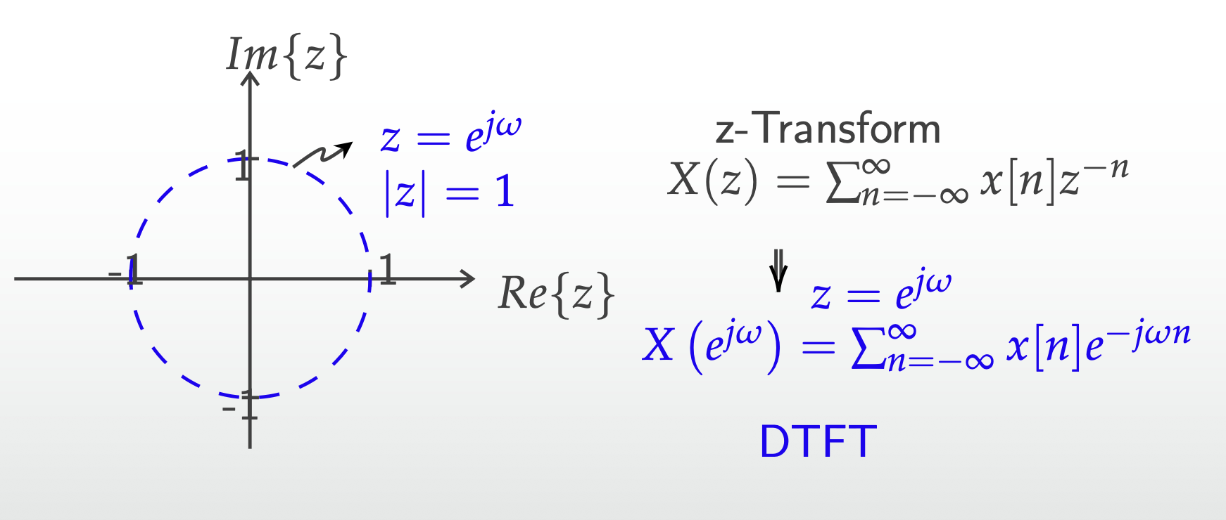
Both are fixed by the same small change. Instead of evaluating the transform only on the unit circle, evaluate it on every circle. Write \(z=re^{j\omega}\) and define
The \(z\)-transform can be viewed as the DTFT of an exponentially weighted sequence \(x[n]r^{-n}\). Choosing \(r\) large enough can make a growing right-sided sequence converge. For example, \(2^n u[n]\) becomes summable after weighting when \(r>2\). Setting \(r=1\) removes the weighting and recovers the DTFT.
Because the weighting depends on \(r\), the transform now exists on some circles and not others. That set of radii is the region of convergence, and Section 4.3 argues it is not a technicality but half of the answer.
A one-sample delay transforms to \(z^{-1}X(z)\). Since a difference equation is a weighted sum of delayed inputs and outputs, the \(z\)-transform converts it into a polynomial equation in \(z^{-1}\). Factoring the resulting numerator and denominator reveals the system's zeros and poles.
The parallel with continuous time is exact, and worth putting side by side because it is the last rung of Lecture 2's ladder:
Continuous time · Lecture 2
$$X(s)=\int x(t)e^{-st}dt$$
CTFT is the special case \(s=j\Omega\): the transform evaluated on the imaginary axis.
Discrete time · this lecture
$$X(z)=\sum_n x[n]z^{-n}$$
DTFT is the special case \(z=e^{j\omega}\): the transform evaluated on the unit circle.
One question remains, and it is the good one: why a circle? In continuous time the Fourier case sits on a straight line; here it sits on a closed curve. Lecture 3 has already supplied the answer.
4.2 Definition, and where the unit circle comes from: \(z=e^{sT}\)
Lecture 1 established that complex exponentials are the eigenfunctions of LTI systems, and Lecture 2 built every transform out of them. So ask what happens to one when it passes through the sampler of Lecture 3. Take \(x(t)=e^{st}\) and sample at \(t=nT\):
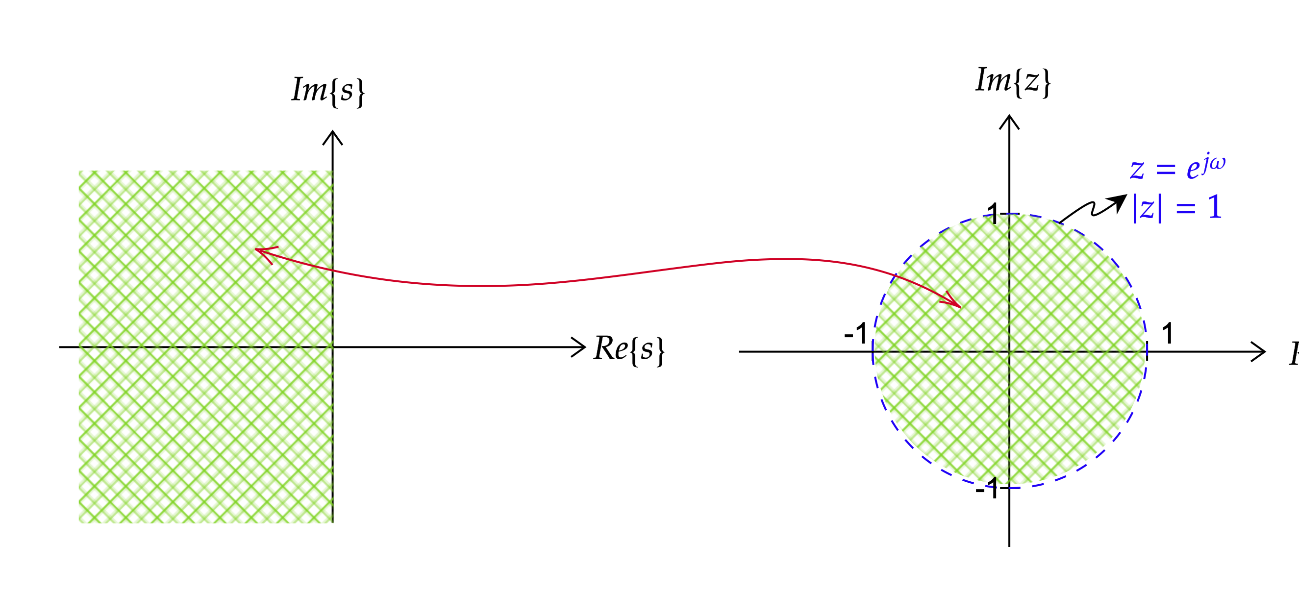
Figure 4.2.a. The map \(z=e^{sT}\), Eq. (4.3). The shaded left half-plane lands inside the shaded unit disk; the \(j\Omega\)-axis wraps onto the unit circle. (Not pictured here, but true of the map: it is many-to-one, since \(e^{sT}\) is periodic in \(\Omega\) with period \(2\pi/T\) — every horizontal strip of that height covers the whole \(z\)-plane, which is why \(\omega\) repeats every \(2\pi\).)
Sampling the continuous-time exponential \(e^{st}\) at \(t=nT\) gives \((e^{sT})^n\). The discrete-time variable is therefore \(z=e^{sT}\). Writing \(s=\sigma+j\Omega\) shows how locations in the \(s\)-plane map into the \(z\)-plane:
Read off the consequences one at a time. They are the three facts Lecture 2 could only tabulate.
\(\sigma<0 \Rightarrow r<1\). The left half-plane maps inside the unit circle. Decaying continuous exponentials sample into decaying discrete ones.
\(\sigma=0 \Rightarrow r=1\). The \(j\Omega\)-axis — the home of the Fourier transform — maps onto the unit circle. That is the answer to the question at the end of Section 4.1: the circle is the image of a straight line under \(e^{sT}\).
\(\omega=\Omega T\). The same exchange rate as Eq. (3.13), arrived at by a different route. Consistency here is not a coincidence — both come from sampling.
The map is periodic in \(\Omega\) with period \(2\pi/T\). Thus, \(s\) and \(s+j2\pi k/T\) map to the same point \(z\). This many-to-one mapping is another view of aliasing and explains why distinct discrete-time frequencies occupy only one \(2\pi\)-radian interval.
Figure 4.2.b. Eq. (4.1) restated: the DTFT is nothing but \(X(z)\) with \(z\) walked around the unit circle, \(z=e^{j\omega}\). This is the same statement as the two-column comparison above, redrawn on the plane it lives in.
4.3 The region of convergence is half the answer
Because Eq. (4.1) is an infinite sum, it converges only in part of the \(z\)-plane. This region of convergence (ROC) is part of the transform. Without it, the algebraic expression \(X(z)\) may correspond to more than one sequence.
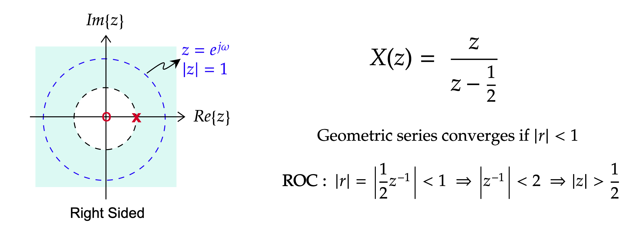
A causal sequence. Let \(x[n]=a^nu[n]\). Then only \(n\ge0\) contributes, and the sum is geometric with ratio \(az^{-1}\):
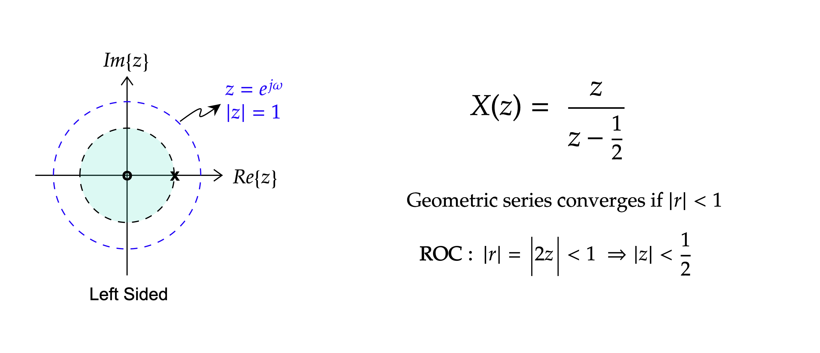
An anti-causal sequence. Now let \(x[n]=-a^nu[-n-1]\), which is zero for \(n\ge0\). Substituting \(k=-n\) turns the sum into a geometric series in \(a^{-1}z\):
Equations (4.5) and (4.6) have the same algebraic expression and the same pole at \(z=a\), but they represent different time-domain sequences. The outward ROC \(|z|>|a|\) gives a right-sided sequence; the inward ROC \(|z|<|a|\) gives a left-sided sequence. Always state the ROC when writing a \(z\)-transform.
4.3.1 Properties of the ROC, and how to infer it
The good news is that you rarely have to derive an ROC. Its shape is heavily constrained, and the constraints let you read it off from a single qualitative fact about the sequence.
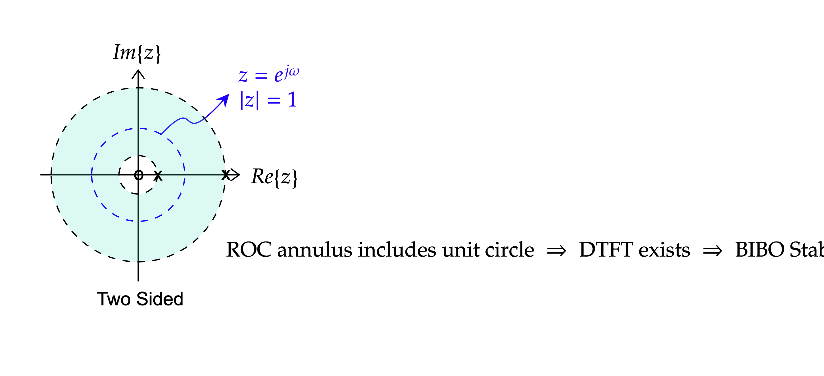
It is always an annulus centred on the origin (possibly degenerate): \(r_{\min}<|z|<r_{\max}\). Convergence depends on \(r\) alone — Eq. (4.2) — never on \(\omega\), so the region cannot be any other shape.
It never contains a pole. By definition the sum blows up there. The boundaries of the ROC are therefore always pole radii.
Right-sided \(\Rightarrow\) outward. If \(x[n]=0\) for \(n<N_1\), the ROC is \(|z|>r_{\max}\): everything outside the outermost pole. Large \(r\) suppresses large positive \(n\), which is where the sequence lives.
Left-sided \(\Rightarrow\) inward. If \(x[n]=0\) for \(n>N_2\), the ROC is \(|z|<r_{\min}\): everything inside the innermost pole.
Two-sided \(\Rightarrow\) an annulus between two poles — or nothing at all, if the inward and outward requirements are incompatible.
Finite-length \(\Rightarrow\) the entire plane, except possibly \(z=0\) or \(z=\infty\). A finite sum always converges.
Figure 4.3.a. The only three shapes an ROC can have, with poles marked \(\times\) and the unit circle dashed. Reading it in reverse is the useful skill: told that a sequence is causal, you already know the ROC is the outward region — and told that a system is stable, you know the region must contain the dashed circle.
In practice, the ROC is often inferred from physical information. If a problem states that a system is causal, the ROC must extend outward beyond the outermost pole. If it states that the system is stable, the ROC must include the unit circle.
EXAMPLE 4.1 · A right-sided sequence, and its ROC
Find \(X(z)\) and its ROC for \(x[n]=\left(\tfrac12\right)^nu[n]\), and say whether a system with this impulse response is stable.
Step 1. Only \(n\ge0\) contributes, so by Eq. (4.5) with \(a=\tfrac12\):
Step 2 \middot; Stability. Right-sided \(\Rightarrow\) the ROC extends outward from the pole, and it already contains \(|z|=1\). So the DTFT exists (Section 4.1) and the system is BIBO stable — this is the ordinary causal, decaying case.
EXAMPLE 4.2 · A left-sided sequence with the identical X(z)
Find \(X(z)\) and its ROC for \(x[n]=-\left(\tfrac12\right)^nu[-n-1]\), and say whether a system with this impulse response is stable.
Step 1. Only \(n\le-1\) contributes, so by Eq. (4.6) with \(a=\tfrac12\):
Step 2 \middot; Stability. The algebra is identical to Example 4.1 — same pole, same \(X(z)\). But this ROC extends inward and excludes \(|z|=1\), so the DTFT does not exist and the system is unstable. Only the shaded region distinguishes the two sequences.
EXAMPLE 4.3 · A two-sided sequence, and why its ROC is an annulus
Find \(X(z)\) and its ROC for \(x[n]=\left(\tfrac12\right)^nu[n]-2^{\,n}u[-n-1]\), and say whether a system with this impulse response is stable.
Step 1. Transform each part separately and intersect the regions — that is all the linearity property allows.
Step 2 \middot; Right-sided part. By Eq. (4.5) with \(a=\tfrac12\):
Step 5 \middot; Stability. The annulus contains \(|z|=1\), so the sequence is absolutely summable there and a system with this impulse response is BIBO stable — even though one pole (at \(z=2\)) lies outside the unit circle. Section 4.4 makes this precise as Eq. (4.7): stability is about the ROC, not about a blanket rule that poles must sit inside the circle — that shortcut (Eq. (4.8)) only holds for causal systems, and this sequence is two-sided. Such a system is stable but not realisable in real time, since it needs future inputs.
A caution about Eq. (4.3)
The relation \(z=e^{sT}\) explains the geometry of the two planes, but it should not be used as a direct substitution to convert any rational \(H(s)\) into \(H(z)\). The exponential mapping is many-to-one and can introduce aliasing. Lecture 8 develops practical mappings, including impulse invariance and the bilinear transform, with their different trade-offs.
4.4 Stability and causality, read off the z-plane
A discrete-time LTI system is BIBO stable when its impulse response is absolutely summable. This is also the condition for its DTFT to converge. Since the DTFT is the \(z\)-transform evaluated at \(r=1\), stability requires the ROC to include the unit circle:
$$\boxed{\;\text{the system is BIBO stable}\iff \text{the ROC of }H(z)\text{ contains the unit circle }|z|=1.\;}$$
(4.7)
For an LTI system, BIBO stability, absolute summability of \(h[n]\), and existence of the ordinary frequency response are therefore linked. If the ROC excludes the unit circle, the DTFT of the impulse response does not converge.
Combine Eq. (4.7) with the causality rule of Section 4.3.1 and the everyday test appears. Causal means the ROC is \(|z|>r_{\max}\); for that outward region to include \(|z|=1\) we need \(r_{\max}<1\):
$$\boxed{\;\text{causal and stable}\iff \text{every pole of }H(z)\text{ satisfies }|p_k|<1.\;}$$
(4.8)
This is the single most-used sentence in digital filter design, and it is worth noticing how weak its hypotheses are. It says nothing about zeros: zeros may sit anywhere, inside, on or outside the circle, without affecting stability. Lecture 7 exploits that freedom heavily.
The s-plane / z-plane correspondence — completing Lecture 2
Concept
Continuous · \(s\)
Discrete · \(z\)
Fourier lives on
the \(j\Omega\)-axis
the unit circle \(|z|=1\)
Stable region
left half-plane \(\sigma<0\)
unit disk \(|z|<1\)
Marginal
poles on \(j\Omega\)
poles on \(|z|=1\)
DC
\(s=0\)
\(z=1\)
Highest frequency
\(\Omega\to\infty\)
\(z=-1\) (i.e. \(\omega=\pi\))
Pure delay
\(e^{-s\tau}\)
\(z^{-1}\) per sample
Integration / accumulation
\(1/s\)
\(1/(1-z^{-1})\)
Every row is a consequence of \(z=e^{sT}\), not a separate convention to memorise. The last two are worth checking against Eq. (4.4) yourself.
Section 4.3's Example 4.3 already worked through a two-sided case in full — the same sequence used there, \(x[n]=\left(\tfrac12\right)^nu[n]-2^{\,n}u[-n-1]\), has one pole inside the unit circle and one outside, yet the annulus \(\tfrac12<|z|<2\) still contains \(|z|=1\). By Eq. (4.7) that system is BIBO stable, even though the causal rule of Eq. (4.8) alone would have said otherwise — a reminder that Eq. (4.8) presumes causality, while Eq. (4.7) is the general criterion.
4.5 Properties, and the standard pairs
The properties mirror Lecture 2's Fourier properties almost line for line, so rather than re-derive them the table below states each with the one thing Fourier did not have to worry about: what happens to the ROC.
Property
Relation
Effect on the ROC
Linearity
\(ax_1[n]+bx_2[n]\leftrightarrow aX_1+bX_2\)
at least the intersection; can be larger if a pole cancels
Time shift
\(x[n-n_0]\leftrightarrow z^{-n_0}X(z)\)
unchanged, except possibly at \(z=0\) or \(\infty\)
initial value needs \(x\) causal; final value needs all poles inside \(|z|=1\) bar one at \(z=1\)
Two of these deserve a sentence more than a table row gives them.
Convolution becomes multiplication: \(Y(z)=H(z)X(z)\). For cascaded filters, the individual system functions multiply, so their poles and zeros combine. This allows high-order filters to be implemented as a cascade of simpler second-order sections, or biquads.
Multiplication by \(a^n\) moves poles and zeros geometrically. Their radii are scaled by \(|a|\), and their angles are shifted by \(\arg a\). When \(a=e^{j\omega_0}\), the movement is a pure rotation, which is useful for shifting a response to a different centre frequency.
Rows 4 and 5 have the same algebraic expression but different regions of convergence, so they represent different sequences. A single complex pole at \(re^{j\omega_0}\) produces a complex exponential. For a real signal, poles occur as the conjugate pair \(re^{\pm j\omega_0}\); adding their contributions gives a real sinusoid. The angle \(\omega_0\) sets the oscillation frequency, and the radius \(r\) sets the factor \(r^n\). As \(r\) moves closer to 1, the oscillation decays more slowly and the system rings for longer.
EXAMPLE 4.4 · A damped sinusoid, transformed with properties instead of sums
Find \(X(z)\), its ROC and its pole–zero pattern for \(x[n]=A\,r^{\,n}\cos(\omega_0 n+\phi)\,u[n]\), with \(0<r<1\). Summing Eq. (4.1) directly is unpleasant; use linearity and Eq. (4.5) instead.
Step 1 · Split the cosine. Euler turns one real sinusoid into two complex exponentials, and each one is a plain geometric sequence:
Step 2 · Transform each term. Eq. (4.5) applies to both, with \(a=re^{\pm j\omega_0}\) and \(|a|=r\) in each case. Linearity adds the transforms and intersects the regions, and here both regions are the same, \(|z|>r\):
Step 3 · Put over a common denominator. The cross terms recombine into cosines, \(e^{j\phi}re^{-j\omega_0}+e^{-j\phi}re^{j\omega_0}=2r\cos(\omega_0-\phi)\), giving a real second-order transform:
Step 4 · Read the plane. The denominator's roots are the conjugate pair \(p_{1,2}=re^{\pm j\omega_0}\): radius \(r\) sets the decay rate of the envelope, angle \(\omega_0\) sets the oscillation frequency. There is one finite zero, at \(z=r\cos(\omega_0-\phi)/\cos\phi\), plus one at the origin, and the phase \(\phi\) moves only that zero, never the poles.
Step 5 · Stability. \(r<1\) puts both poles inside the unit circle, so the ROC \(|z|>r\) contains \(|z|=1\) and the sequence is absolutely summable, exactly as Eq. (4.7) requires.
Keep this denominator in mind: \(1-2r\cos\omega_0z^{-1}+r^2z^{-2}\) is the two-pole resonator of Lecture 6 (Eq. 6.6). A decaying sinusoid and a resonant filter are the same pair of poles read in two directions — one as a signal, one as a system.
4.6 Getting back: three ways to invert
There is a formal inversion formula — a contour integral counter-clockwise around a closed path inside the ROC,
evaluated by residues. The contour must lie inside the ROC, which shows mathematically why a different ROC gives a different time sequence. For routine engineering problems, inspection, partial fractions and power-series expansion are usually more convenient.
4.6.1 Inspection, and partial fractions
If \(X(z)\) is rational — and for any LCCDE system it is — split it into first-order pieces and read each off the table. Two mechanical cautions cause most of the lost marks:
Mind the extra \(z\). The table's pairs have a \(z\) in the numerator: \(z/(z-a)\), not \(1/(z-a)\). A term \(A/(z-a)\) is \(Az^{-1}\cdot z/(z-a)\), and the \(z^{-1}\) is a one-sample delay by the shift property — so the answer is \(Aa^{n-1}u[n-1]\), not \(Aa^nu[n]\). Alternatively, do the partial fractions in \(z^{-1}\) from the start and the problem does not arise.
Repeated poles need every order. A double pole at \(a\) needs both \(A/(z-a)\) and \(B/(z-a)^2\); the second inverts to \(n a^n u[n]\) by the differentiation property, giving the characteristic \(n\,r^n\) growth-then-decay.
Then — and only then — use the ROC to decide the direction of each term. This is the step students skip, and Example 4.5 is entirely about it.
EXAMPLE 4.5 · One X(z), three ROCs, three different sequences
Invert \(X(z)=\dfrac{z}{(z-\tfrac12)(z-2)}\) for each of the three possible ROCs.
Step 1 · Partial fractions. Write \(X(z)=\dfrac{A}{z-\tfrac12}+\dfrac{B}{z-2}\). Multiplying up, \(z=A(z-2)+B(z-\tfrac12)\). By residues: \(A=\left.\dfrac{z}{z-2}\right|_{z=1/2}=\dfrac{1/2}{-3/2}=-\tfrac13\), and \(B=\left.\dfrac{z}{z-\tfrac12}\right|_{z=2}=\dfrac{2}{3/2}=\tfrac43\).
Step 2 · Restore the numerator \(z\). Each term is \(A/(z-a)=Az^{-1}\cdot z/(z-a)\), so by the shift property every inverse acquires a one-sample delay:
$$\frac{A}{z-a}\;\longleftrightarrow\;A\,a^{\,n-1}u[n-1]\quad\text{(if taken causally)}.$$
Step 3 · The ROC decides each term's direction. The poles are at \(\tfrac12\) and \(2\), so three regions are possible:
\(|z|>2\)
outside both poles \(\Rightarrow\) both terms causal, right-sided: \(x[n]=\left[-\tfrac13(\tfrac12)^{n-1}+\tfrac43 2^{\,n-1}\right]u[n-1]\). Contains no unit circle → unstable, and it grows without bound.
\(|z|<\tfrac12\)
inside both \(\Rightarrow\) both anti-causal, left-sided: \(x[n]=\left[\tfrac13(\tfrac12)^{n-1}-\tfrac43 2^{\,n-1}\right]u[-n]\). Also excludes \(|z|=1\) → unstable.
\(\tfrac12<|z|<2\)
outside the \(\tfrac12\) pole, inside the \(2\) pole \(\Rightarrow\) two-sided: the \(\tfrac12\) term causal, the \(2\) term anti-causal. Contains \(|z|=1\) → stable.
Step 4. Three completely different signals — one growing forward, one growing backward, one decaying in both directions — from one algebraic expression. The rule to carry away: a pole contributes causally if the ROC is outside it, anti-causally if the ROC is inside it. Decide per pole, not per problem.
MATLAB corner for Example 4.5
A rational expression in \(z\) does not identify a unique sequence unless its region of convergence is also known. MATLAB's standard impulse-response functions assume a causal system, so the script constructs the anti-causal sequence separately. Comparing the two results makes the role of the ROC explicit.
Goal: plot the causal and anti-causal sequences that share one \(X(z)\), and confirm which one is absolutely summable, then verify Example 4.5's three inversions numerically.
roc_decides.m
MATLAB
%% Same X(z), two ROCs, two sequences (Section 4.3)
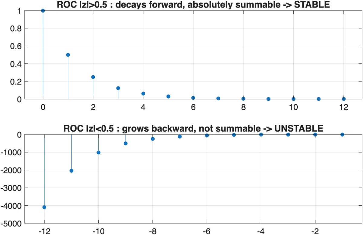
Figure 4.6.Reading the MATLAB comparison. Both plots use the same algebraic expression, \(X(z)=1/(1-0.5z^{-1})\), so the coefficient vectors alone cannot distinguish them. For the ROC \(|z|>0.5\), the sequence is right-sided: \((0.5)^n u[n]\). It decays as \(n\) increases and is absolutely summable. For \(|z|<0.5\), the sequence is left-sided: \(-(0.5)^n u[-n-1]\). Its samples grow as time moves towards \(-\infty\), so it is not absolutely summable. The ROC therefore determines both time direction and stability.
4.6.2 Power series, when the transform is not rational
Eq. (4.1) says \(X(z)\) is a power series in \(z^{-1}\) whose coefficients are the samples. So any expansion valid in the ROC identifies \(x[n]\) directly by matching coefficients — no factoring, no table.
The ROC decides which expansion is legal, and this is where the method earns its keep. For \(X(z)=1/(1-\tfrac12z^{-1})\):
ROC \(|z|>\tfrac12\)
Expand in negative powers, since \(|\tfrac12z^{-1}|<1\):
Coefficients give \(x[n]=(\tfrac12)^nu[n]\) — causal.
ROC \(|z|<\tfrac12\)
Now \(|2z|<1\), so rearrange and expand in positive powers:
$$-2z\sum_{k=0}^{\infty}(2z)^{k}$$
Positive powers of \(z\) sit at negative \(n\): \(x[n]=-(\tfrac12)^nu[-n-1]\) — anti-causal.
Power-series expansion also works for non-rational transforms. For example, \(e^{z^{-1}}=\sum_k z^{-k}/k!\) immediately gives \(x[n]=1/n!\) for \(n\ge0\). The method may produce only a sequence of coefficients rather than a compact formula, but that is often enough when only the first few impulse-response samples are required.
EXAMPLE 4.6 · A transform that is not rational, inverted two ways
Find \(x[n]\) for \(X(z)=\log\!\left(1-az^{-1}\right)\), \(|z|>|a|\). There are no poles and zeros to expand, so partial fractions has nothing to work with.
Method 1 · Power series. Inside the ROC \(|az^{-1}|<1\), so the standard series \(\log(1-u)=-\sum_{k\ge1}u^{k}/k\) is legal with \(u=az^{-1}\):
That is a first-order transform: by Eq. (4.5) and the shift property its inverse is \(-a^{\,n}u[n-1]\). So \(n\,x[n]=-a^{\,n}u[n-1]\), and dividing by \(n\) recovers the same answer — a useful check that the series was expanded in the right variable.
Two lessons. First, the ROC still decides everything: expanding in powers of \(z\) instead of \(z^{-1}\) would have produced the left-sided answer, valid for \(|z|<|a|\). Second, non-rational transforms are not exotic — they appear whenever a system is described by a logarithm or an exponential, and the power-series method is the only one of the three that reaches them.
4.7 Difference equations become algebra: LCCDEs, FIR and IIR
Here is the payoff that motivated the transform in the first place. A great many discrete systems — every digital filter, every discrete controller, every recursive average — are described by a linear constant-coefficient difference equation:
Now transform Eq. (4.10). Every delay \(y[n-k]\) becomes \(z^{-k}Y(z)\), the sums come out of the transform by linearity, and what was a recursion in time is a single algebraic equation. Dividing:
The \(q_m\) are the zeros: frequencies the filter kills. The \(p_k\) are the poles: frequencies it emphasises. Designing a filter is choosing where to put these points, and Eq. (4.8) constrains the poles to the interior of the unit circle.
A common confusion, stated plainly
The zeros of \(H(z)\) are the roots of its numerator, and its poles are the roots of its denominator. They describe the system itself. Do not confuse them with poles or zeros that may appear in the input \(X(z)\) or output \(Y(z)\).
4.7.1 Recursive or not: IIR and FIR
Eq. (4.11) splits the world in two, on one question: does the output depend on past outputs?
\(N=0\) · non-recursive · FIR
No feedback: \(y[n]=\sum_{m}b_mx[n-m]\). The impulse response is the coefficient list, \(h[n]=b_n\), and it stops after \(M+1\) samples — hence finite impulse response.
All poles sit at \(z=0\), so an FIR filter is always stable, whatever the coefficients. It can also be made exactly linear-phase. Lecture 7.
\(N\ge1\) · recursive · IIR
With feedback, each output re-enters the computation forever. Unless the coefficients contrive an exact cancellation, \(h[n]\) never truly reaches zero — an infinite impulse response from a handful of coefficients.
Far more selective per coefficient, but it has genuine poles, so stability must be checked — Eq. (4.8). Lecture 8.
That trade — guaranteed stability and linear phase against efficiency — is the central engineering decision of the second half of this module, and it is visible entirely in \(N\).
4.7.2 Zero-input and zero-state response
A recursive system has memory, so its output has two independent causes, and the transform keeps them apart:
$$ y[n]=y_{\text{ZI}}[n]+y_{\text{ZS}}[n]. $$
(4.14)
The zero-input response is caused by the system's initial stored state when the external input is zero. It is the homogeneous solution and is built from the natural modes \(p_k^n\). The zero-state response is the response to the input when all initial conditions are zero: \(y_{\text{ZS}}=x*h\), or \(Y_{\text{ZS}}(z)=H(z)X(z)\).
Note which one the poles govern: both. The homogeneous solution's terms are exactly \(p_k^{\,n}\), so if every \(|p_k|<1\) any initial-condition transient dies out on its own. That is the time-domain meaning of Eq. (4.8) — a stable filter forgets its own startup state.
4.7.3 Realization: three blocks, and that is all
Eq. (4.11) needs an adder, a constant multiplier and a one-sample delay. Nothing else. Every filter structure in this module is those three components wired differently, and the wiring diagram is a faithful picture of the arithmetic a processor performs per sample.
Figure 4.7. (a) The three primitives. (b) A second-order section in direct form II: the feedback (\(-a_k\)) taps run above the delay chain and the feed-forward (\(b_m\)) taps below, so a single chain of delays serves both. This halves the storage of the obvious arrangement — two delays rather than four — and is why biquads are written this way in practice.
The number of delays is the filter's order, and it is what costs memory; the multipliers are what cost arithmetic. Reading a structure for those two counts is how implementations are compared.
4.8 The geometric method: seeing \(|H(e^{j\omega})|\) in the z-plane
The pole–zero plot gives a visual way to estimate a filter's frequency response. It also provides a design guide: place poles near frequencies to be emphasized and zeros near frequencies to be suppressed.
Start from the factored form, Eq. (4.13), and evaluate it on the unit circle:
Every factor has the form \((e^{j\omega}-c)\), which is a vector in the complex plane: it points from the fixed point \(c\) to the moving point \(e^{j\omega}\) on the unit circle. Taking magnitudes and angles of Eq. (4.15) separates cleanly:
$$\boxed{\;\left|H(e^{j\omega})\right|=|b_0|\,\frac{\prod_m\big(\text{length from zero }q_m\big)}{\prod_k\big(\text{length from pole }p_k\big)}\;}$$
(4.16)
$$ \angle H(e^{j\omega})=\omega(N-M)+\sum_m\big(\text{angle of zero vector}\big)-\sum_k\big(\text{angle of pole vector}\big). $$
(4.17)
So: walk the point \(e^{j\omega}\) once around the unit circle and watch the rubber bands stretch. Where a pole vector gets short, \(|H|\) rises. Where a zero vector gets short, \(|H|\) falls. Nothing needs to be computed to know the shape.
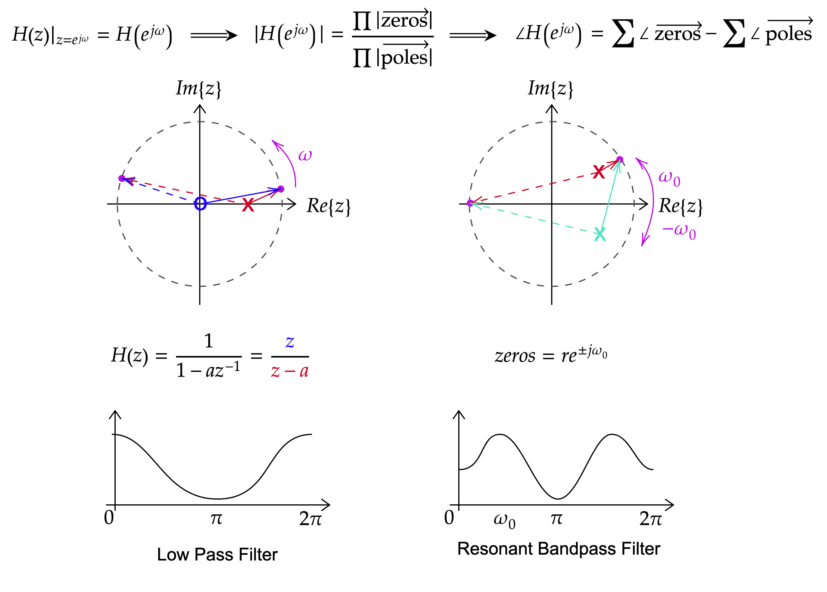
Figure 4.8.a. Two worked cases of Eq. (4.16). Left: a single real pole at \(z=a\), \(H(z)=z/(z-a)\) — as \(\omega\) rotates, the vector from the pole shortens near \(\omega=0\), giving the low-pass shape below. Right: a conjugate pole pair at \(re^{\pm j\omega_0}\) — the vector from the upper pole shortens near \(\omega=\omega_0\), producing the resonant bandpass peak; the zeros near the origin barely affect either curve.
Three consequences do most of the work in practice.
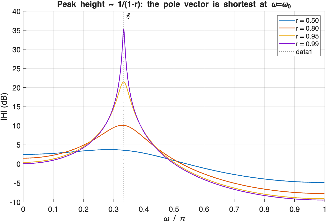
A pole at radius \(r\) and angle \(\theta\) makes a peak at \(\omega=\theta\), and its sharpness is governed by \(1-r\). At the closest approach the pole vector has length \(1-r\), so the peak height goes as \(1/(1-r)\): a pole at \(r=0.99\) gives a peak ten times taller and far narrower than one at \(r=0.9\). Resonance is proximity to the circle.
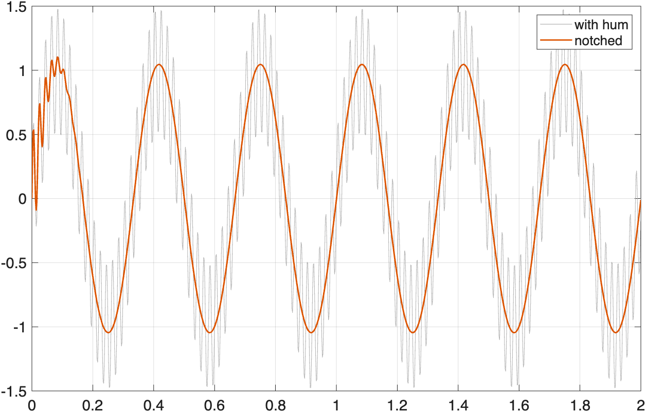
A zero on the circle at \(e^{j\omega_0}\) forces \(|H(e^{j\omega_0})|=0\) exactly — a perfect null. That is how a notch filter removes mains hum: place a zero pair at \(\omega_0=2\pi f_0/f_s\). A zero merely near the circle gives a finite dip.
Distance mutes influence. A pole or zero near the origin is roughly the same distance from every point on the circle, so it contributes an almost constant factor and hardly shapes the response at all. Only features near the circle matter — which is why pole–zero plots are read radially outward.
Figure 4.8.b. Four filters, each as a pole–zero plot (above) and the \(|H(e^{j\omega})|\) it produces for \(\omega:0\to\pi\) (below). The whole catalogue follows from the two rules: a pole near \(z=+1\) boosts low frequencies; the same pole near \(z=-1\) boosts high ones; zeros on the circle punch exact nulls; a pole pair just inside the circle rings at its own angle. Lectures 7–8 are systematic ways of choosing these locations to meet a specification.
EXAMPLE 4.7 · Designing a 50 Hz notch by placing four points
An ECG sampled at \(f_s=500\,\text{Hz}\) is contaminated by \(50\,\text{Hz}\) mains hum. Design a second-order notch that removes it while disturbing the rest of the band as little as possible. Give the difference equation.
Step 1 · Where is 50 Hz on the circle? By Eq. (3.13), \(\omega_0=2\pi f_0/f_s=2\pi(50)/500=0.2\pi\) rad/sample \(=36^{\circ}\).
Step 2 · Kill it with zeros. Section 4.8 says a zero exactly on the circle gives an exact null, so place a conjugate pair at \(e^{\pm j0.2\pi}\):
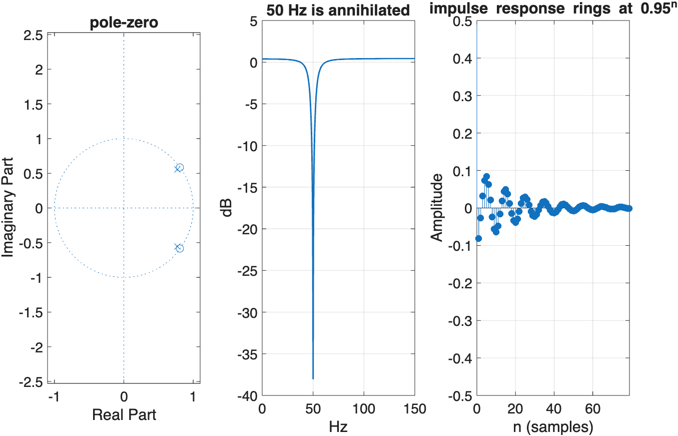
Step 3 · Narrow the notch with poles. Zeros alone give a wide, shallow-sided dip that removes wanted signal either side of \(50\,\text{Hz}\). Put a pole pair at the same angle but just inside the circle, \(r=0.95\): away from \(\omega_0\) each pole vector nearly cancels its neighbouring zero vector, so \(|H|\approx1\) across the rest of the band, while at \(\omega_0\) the zero still wins absolutely.
Five multiplies and four delays — and the poles are at \(|p|=0.95<1\), so by Eq. (4.8) it is stable. Push \(r\) to \(0.99\) for a narrower notch, at the cost of a longer ringing transient (the impulse response decays as \(0.99^n\)). That trade — selectivity against time-domain settling — is unavoidable, and it is Lecture 8's recurring theme.
MATLAB corner for Example 4.5
This script makes Section 4.8 tangible: drag a pole outward and watch the resonance peak sharpen, then builds the Example 4.7 notch and shows it three ways — pole–zero plot, magnitude response, and difference-equation output — from the same coefficients.
Goal: sweep the pole radius \(r\) toward the unit circle to see the peak height and width track \(1/(1-r)\), then reproduce Example 4.5's notch from its pole–zero placement.
pole_zero_explorer.m
MATLAB
%% L4_2_fixed.m
%% Part 1 - resonance IS proximity to the unit circle (Eq. 4.16)
w0 = pi/3;
figure('Color','w'); hold on; grid on;
for r = [0.50.80.950.99]
b = 1;
a = [1, -2*r*cos(w0), r^2];
[H,w] = freqz(b, a, 1024);
plot(w/pi, 20*log10(abs(H)), 'LineWidth',1.5, ...
'DisplayName', sprintf('r = %.2f', r));
end
xline(w0/pi, 'k:', '\omega_0'); legend show;
xlabel('\omega / \pi'); ylabel('|H| (dB)');
title('Peak height ~ 1/(1-r): the pole vector is shortest at \omega=\omega_0');
isstable(tf(b, a_bad, 1/fs)); % requires Control System Toolbox
Figure 4.8.c.How to read the MATLAB explorer. In the top row, the pole angle fixes the resonant frequency \(\omega_0\). Increasing the pole radius \(r\) moves the poles closer to the unit circle, so the resonance becomes taller and narrower; its centre frequency does not move. The middle row shows the notch design from three linked views: pole–zero map, magnitude response and phase. Zeros on the unit circle at the unwanted frequency force the magnitude to zero there, while nearby poles control the notch width. In the time-domain result at the bottom, the 50 Hz component is suppressed and the 3 Hz component remains. The short ringing at the start is the filter transient produced by the nearby poles.
4.9 Closing the ladder: what each transform was for
The transforms introduced so far form a connected family rather than six unrelated formulas. The Laplace transform is the general continuous-time transform, and the \(z\)-transform is its discrete-time counterpart. The Fourier transforms are obtained by evaluating these general transforms on particular boundaries.
The whole toolkit, on one page
Transform
Is really
Reach for it when
Laplace \(X(s)\)
the general CT transform
analog circuits, stability, transients
CTFT \(X(j\Omega)\)
Laplace on the \(j\Omega\)-axis
steady-state spectra of analog signals
CTFS \(X_k\)
CTFT of a periodic signal — lines
periodic waveforms, harmonics
\(z\) \(X(z)\)
the general DT transform
filter design, difference equations, stability
DTFT \(X(e^{j\omega})\)
\(z\) on the unit circle
frequency response of a stable system
DFT \(X[k]\)
DTFT sampled at \(N\) points
actual computation, via the FFT
Read each side from the general transform to its Fourier restriction and then to a finite computational form. The mapping \(z=e^{sT}\) connects the continuous- and discrete-time sides through sampling.
The choice of transform depends on whether the signal is continuous or discrete and whether the task is theoretical analysis, frequency-response measurement or finite computation.
The next lectures use this toolkit for filter design. Lecture 5 develops analog prototypes, Lecture 7 designs FIR filters, and Lecture 8 maps analog designs into digital IIR filters. In each case, the goal is to place poles and zeros so that selected frequencies pass while others are attenuated.
?Problems with solutions
PROBLEM 4.1
Which of these sequences have a convergent DTFT? For each, give the ROC of its \(z\)-transform. (i) \(2^nu[n]\) (ii) \(2^nu[-n]\) (iii) \((\tfrac12)^nu[n]\) (iv) \(u[n]\).
Solution. The DTFT converges iff \(\sum|x[n]|<\infty\) iff the ROC contains \(|z|=1\) — Eq. (4.7). So one test answers both halves.
(i)
\(|z|>2\)
right-sided, grows as \(2^n\). Excludes the unit circle → no DTFT.
(ii)
\(|z|<2\)
left-sided; as \(n\to-\infty\), \(2^n\to0\), so it decays going backward and is summable. Contains \(|z|=1\) → DTFT exists. Note this is the mirror of (i): the same base, opposite side, opposite verdict.
(iii)
\(|z|>\tfrac12\)
right-sided and decaying → DTFT exists.
(iv)
\(|z|>1\)
the pole sits on the circle, so the ROC is open at \(|z|=1\) and excludes it → no DTFT in the ordinary sense. (Lecture 2 gave it one only by admitting an impulse at \(\omega=0\) — the marginal case, and exactly why marginal stability is not stability.)
PROBLEM 4.2
\(X(z)\) has poles at \(z=\tfrac13,\,2,\,3\) and no others. (a) If the DTFT of \(x[n]\) is known to converge, what is the ROC, and is \(x[n]\) right-, left- or two-sided? (b) If instead it is known only that \(x[n]\) is two-sided, how many different sequences could this pole pattern correspond to?
(a) The pole radii \(\tfrac13,2,3\) cut the plane into four candidate annuli: \(|z|<\tfrac13\), \(\tfrac13<|z|<2\), \(2<|z|<3\), \(|z|>3\). A convergent DTFT means the ROC contains \(|z|=1\), and only \(\tfrac13<|z|<2\) does.
That region is an annulus with poles on both boundaries, so \(x[n]\) is two-sided: the \(\tfrac13\) pole lies inside the ROC boundary and contributes a causal term, while the poles at \(2\) and \(3\) lie outside it and contribute anti-causal terms.
(b) Of the four annuli, the two extremes are not two-sided: \(|z|>3\) is right-sided and \(|z|<\tfrac13\) is left-sided. The two interior annuli — \(\tfrac13<|z|<2\) and \(2<|z|<3\) — are both bounded by poles on either side, so both give two-sided sequences. Answer: two.
Worth noticing how much was determined by two words. “The DTFT converges” pinned the region uniquely out of four; “two-sided” narrowed it to two. This is what Section 4.3.1 meant by inferring the ROC rather than deriving it.
PROBLEM 4.3
A causal system has \(H(z)=\dfrac{z^{-1}-a}{1-az^{-1}}\) with \(a\) real, \(0<a<1\). Show geometrically that \(|H(e^{j\omega})|\) is constant — an all-pass filter.
Locate the pole and zero. Multiply numerator and denominator by \(z\): \(H(z)=\dfrac{1-az}{z-a}\), so there is a pole at \(z=a\) and a zero at \(z=1/a\). Since \(0<a<1\), the pole is inside the circle and the zero is outside it, at the reciprocal radius, on the same ray. The ROC is \(|z|>a\) (causal), which contains \(|z|=1\) → stable.
The geometric argument. Take any point \(e^{j\omega}\) on the circle and form the two vectors. The claim is that their length ratio does not depend on \(\omega\). Compute both squared lengths:
They are identical. Hence \(|H(e^{j\omega})|=1\) for every \(\omega\): however the point moves, the zero vector and the pole vector stretch by exactly the same amount, and the ratio in Eq. (4.16) never changes.
Why it matters. A pole–zero pair at reciprocal radii \(a\) and \(1/a\) is an all-pass section: it alters phase only. That gives two standard tools — correcting the phase of an otherwise acceptable magnitude response, and building fractional-delay and phase-equalising structures. It also shows that magnitude does not determine a filter: you may cascade any number of all-pass sections without touching \(|H|\) at all.
PROBLEM 4.4
A stable system obeys \(y[n-1]-\tfrac{5}{2}y[n]+y[n+1]=x[n]\). Find its impulse response. (Note the \(y[n+1]\): the equation as written is not causal.)
Transform. Using \(y[n-1]\to z^{-1}Y\) and \(y[n+1]\to zY\):
Factor. \(z^2-\tfrac52z+1=(z-2)(z-\tfrac12)\), so there are poles at \(z=2\) and \(z=\tfrac12\) — one outside the unit circle, one inside.
Use stability to pick the ROC. Three annuli are available; only \(\tfrac12<|z|<2\) contains \(|z|=1\). Stability therefore forces a two-sided impulse response — consistent with the non-causal \(y[n+1]\) term. There is no causal stable solution here.
Invert. By residues, \(H(z)=\dfrac{z}{(z-2)(z-\frac12)}\) has \(A=\left.\frac{z}{z-\frac12}\right|_{z=2}=\tfrac43\) at \(z=2\) and \(B=\left.\frac{z}{z-2}\right|_{z=1/2}=-\tfrac13\) at \(z=\tfrac12\). The \(\tfrac12\) pole is inside the ROC boundary → causal; the \(2\) pole is outside → anti-causal:
Both halves decay away from the origin — \((\tfrac12)^n\) forward, \(2^n\) backward — so \(\sum|h[n]|<\infty\) as required. This is Section 4.3.1 doing real work: the word “stable” in the question was the only thing that made the answer unique.
PROBLEM 4.5
A causal FIR filter has \(h[n]=1\) for \(0\le n\le N-1\) and zero otherwise — the moving-sum, or “boxcar”. Find \(H(z)\), its poles and zeros, and explain the shape of \(|H(e^{j\omega})|\) geometrically. Where do the nulls fall?
Poles and zeros. The numerator \(z^N-1\) vanishes at the \(N\) roots of unity, \(z=e^{j2\pi k/N}\). The denominator gives a pole at \(z=1\) and an \((N-1)\)-fold pole at the origin. But \(k=0\) puts a zero at \(z=1\) as well, and it cancels the pole there — as it must, since a finite-length sequence cannot have a pole anywhere but the origin (Section 4.3.1). What is left is \(N-1\) zeros spread evenly around the unit circle at
$$z=e^{j2\pi k/N},\qquad k=1,2,\dots,N-1,$$
and all poles at the origin — so it is stable for any \(N\), as every FIR filter is.
Geometric reading. The poles at the origin are equidistant from the whole circle and so contribute nothing to the shape (Section 4.8, third rule). Only the zeros matter, and there is one every \(2\pi/N\) radians — except at \(\omega=0\), where the gap left by the cancelled zero produces the main lobe. So:
nulls at
\(\omega_k=2\pi k/N\), \(k=1,\dots,N-1\) — exactly on the zeros
peak at
\(\omega=0\), where \(H(1)=N\): the widest gap between zeros
shape
a main lobe of width \(\sim4\pi/N\) with \(N-2\) sidelobes between the nulls
Substituting \(z=e^{j\omega}\) and simplifying confirms it: \(|H|=\left|\dfrac{\sin(N\omega/2)}{\sin(\omega/2)}\right|\), the Dirichlet kernel. Note that this is the same function that appeared as the DTFT of a rectangular window in Lecture 2 — and it is why a plain moving average is a mediocre low-pass filter: its sidelobes are only about \(13\,\text{dB}\) down. Fixing that is precisely what windowing does in Lecture 7.
PROBLEM 4.6
Let \(x[n]\) be causal with \(x[0]\neq0\). (a) Show that \(\lim_{z\to\infty}X(z)=x[0]\). (b) Hence show that a rational \(X(z)\) has neither a pole nor a zero at \(z=\infty\), and that it therefore has equally many finite poles and finite zeros. (c) State the corresponding limit for a sequence that is zero for \(n>0\).
(a) Initial-value theorem. Causality kills every negative-\(n\) term of Eq. (4.1), leaving
$$X(z)=x[0]+x[1]z^{-1}+x[2]z^{-2}+\cdots$$
Every term beyond the first carries a factor \(z^{-n}\) with \(n\ge1\), and each vanishes as \(|z|\to\infty\). The ROC of a causal sequence extends outward to infinity (Section 4.3.1), so the limit is taken inside the region where the series converges and may be taken term by term. Hence \(\lim_{z\to\infty}X(z)=x[0]\).
(b) No pole, no zero at infinity. The limit exists (no pole) and equals \(x[0]\neq0\) (no zero). Now write the rational transform as a ratio of polynomials in \(z\), of degrees \(M\) in the numerator and \(N\) in the denominator. For large \(|z|\) the leading terms dominate, so \(X(z)\sim c\,z^{M-N}\). A finite non-zero limit forces \(M-N=0\): the numbers of finite zeros and finite poles are equal. Counting the \((N-1)\)-fold pole at the origin is what makes an FIR filter obey this too — see Problem 4.5's boxcar.
(c) Reverse the roles. If \(x[n]=0\) for \(n>0\), only non-positive powers survive, the ROC extends inward to the origin, and \(\lim_{z\to0}X(z)=x[0]\).
PROBLEM 4.7
Starting from the definition, prove that (i) \(x[-n]\leftrightarrow X(1/z)\) and (ii) \(n\,x[n]\leftrightarrow-z\,dX(z)/dz\), stating what happens to the ROC in each case. Then use (ii) to write down the transform of \(n\,a^{\,n}u[n]\).
(i) Time reversal. Substitute \(m=-n\) in the defining sum:
The ROC inverts with it: if \(X(z)\) converges for \(r_1<|z|<r_2\), then \(X(1/z)\) converges for \(1/r_2<|z|<1/r_1\). Reversing a right-sided sequence makes it left-sided, and the annulus turns inside out to match.
(ii) Differentiation. Differentiate Eq. (4.1) term by term, which a power series permits anywhere strictly inside its ROC:
which is exactly the second-order term Section 4.6.1 warned about: a repeated pole inverts to a sequence carrying a factor of \(n\), so a double pole on the unit circle is not marginally stable but unbounded.
PROBLEM 4.8
Which of these could be the system function of a causal system (stable or not)? Give the reason, not just the verdict. (a) \(\dfrac{(1-z^{-1})^{2}}{1-\tfrac12z^{-1}}\) (b) \(\dfrac{(z-1)^{2}}{z-\tfrac12}\) (c) \(\dfrac{(z-\tfrac14)^{5}}{(z-\tfrac12)^{6}}\) (d) \(\dfrac{(z-\tfrac14)^{6}}{(z-\tfrac12)^{5}}\)
The test. Causal means \(h[n]=0\) for \(n<0\), so by Problem 4.6 the ROC must reach out to \(z=\infty\) and \(H(z)\) must stay finite there. In terms of degrees in \(z\): the numerator degree must not exceed the denominator degree. Equivalently, written in \(z^{-1}\), no positive powers of \(z\) may appear.
(a) yes
already in \(z^{-1}\) with no positive powers; \(H(z)\to1\) as \(z\to\infty\). Causal, and stable too since the only pole is at \(\tfrac12\).
(b) no
degree 2 over degree 1, so \(H(z)\sim z\to\infty\): a pole at infinity. Dividing out gives a term in \(z\), whose inverse is \(\delta[n+1]\) — an output one sample before the input.
(c) yes
degree 5 over degree 6, \(H(\infty)=0\). A zero at infinity is harmless; only a pole there breaks causality.
(d) no
degree 6 over degree 5, again a pole at infinity.
Notice what the test is not about: pole radii decide stability, the degree comparison decides causality. Case (a) has both; a version of (a) with its pole moved to \(z=2\) would still be causal, just unstable.
PROBLEM 4.9
From \(x[n]\) build \(x_1[n]=x[n/M]\) when \(n\) is a multiple of \(M\) and \(x_1[n]=0\) otherwise — the original samples with \(M-1\) zeros stuffed between each pair. (a) Express \(X_1(z)\) in terms of \(X(z)\). (b) If \(X(e^{j\omega})\) is a low-pass shape occupying \(|\omega|<\omega_c\), sketch \(X_1(e^{j\omega})\) for \(M=2\).
(a) Only the multiples of \(M\) contribute, so put \(n=mM\):
with the ROC scaled accordingly: if \(X(z)\) converges for \(r_1<|z|<r_2\), then \(X_1(z)\) converges for \(r_1^{1/M}<|z|<r_2^{1/M}\). Zero-stuffing costs nothing in the transform: it just relabels the exponent.
(b) On the unit circle this reads \(X_1(e^{j\omega})=X(e^{j\omega M})\), so the spectrum is compressed by the factor \(M\) along \(\omega\). For \(M=2\) the original band \(|\omega|<\omega_c\) shrinks to \(|\omega|<\omega_c/2\), and because \(X\) is \(2\pi\)-periodic a second, complete copy of the band appears centred at \(\omega=\pi\). One period of \(X_1\) therefore shows two copies where \(X\) showed one.
That extra copy is an image, and it is the same phenomenon Lecture 3 met from the other direction: sampling replicates a spectrum, and inserting zeros is sampling's mirror image in the discrete domain. Removing the image is the job of the low-pass interpolation filter in any upsampler.
Summary and key formulas
The reference sheet: definition, geometry, stability and the route from a difference equation to a frequency response.
The \(z\)-transform is the DTFT of \(x[n]r^{-n}\). That one sentence explains why it exists where the DTFT does not, and why the DTFT is the special case \(r=1\) — the unit circle.
\(z=e^{sT}\), straight from sampling \(e^{st}\). Hence \(\sigma<0\mapsto|z|<1\), the \(j\Omega\)-axis \(\mapsto\) the unit circle, \(\omega=\Omega T\), and — because \(e^{sT}\) is periodic — a many-to-one map, which is aliasing restated.
The ROC is half the answer. \(a^nu[n]\) and \(-a^nu[-n-1]\) have identical \(X(z)\) and identical poles; only the region distinguishes them. Right-sided \(\Rightarrow\) outward, left-sided \(\Rightarrow\) inward, two-sided \(\Rightarrow\) an annulus, finite \(\Rightarrow\) everywhere.
Stability, absolute summability and existence of a frequency response are one condition: the ROC contains \(|z|=1\). Add causality and it becomes the familiar all poles inside the unit circle. Zeros are unconstrained.
Because a delay is \(z^{-1}\), an LCCDE becomes a rational \(H(z)\). \(N=0\) means FIR — poles only at the origin, unconditionally stable; \(N\ge1\) means IIR — efficient, but stability must be checked.
Invert by inspection and partial fractions when \(X(z)\) is rational (watch the numerator \(z\), and let the ROC choose each term's direction), and by power series when it is not.
The geometric method is the skill to keep: \(|H|\) is the product of zero-vector lengths over pole-vector lengths. Poles near the circle make peaks of height \(\sim1/(1-r)\); zeros on it make exact nulls; anything near the origin barely matters.
Next, in Lecture 5: classical analog filter design — Butterworth, Chebyshev and elliptic prototypes, and the specification language (passband ripple, stopband attenuation, transition width) that Lectures 7 and 8 will translate into pole and zero positions on the plane you have just learned to read.
 MATLAB corner for Example 4.5