ELEC6218 · Signal Processing Analog & Digital Filter Design
Signal Processing · Lecture notes Prof. Çelik
ELEC6218 · Signal Processing
Lecture 2

The Transform Toolkit

This lecture connects time-domain equations with frequency-domain tools. You will use the Laplace transform to obtain transfer functions, poles and stability information. You will then see how the CTFT, CTFS, DTFT and DTFS describe different signal types, and how the DFT and FFT make frequency analysis practical on a computer.

Quiz
Podcast
InstructorProf. Abdulkadir Çelik (https://akadircelik.com) ModuleELEC6218 TopicsLaplace · poles & stability · CTFT · CTFS · DTFT · DTFS · DFT & FFT
▸ Laplace → Fourier ▸ Complex exponentials ▸ The Fourier ladder ▸ DFT & FFT
Learning outcomes

By the end of this lecture, you will be able to:

  • Derive \(H(s)\) from a differential equation, invert it using partial fractions, and assess BIBO stability from its poles.
  • Explain how the CTFT is obtained by evaluating the Laplace transform on the \(j\Omega\)-axis and why complex exponentials are eigenfunctions of LTI systems.
  • Choose the correct transform—CTFT, CTFS, DTFT or DTFS—for a signal's time-domain properties.
  • Use transform properties, calculate a Fourier series and a small DFT, and explain why the FFT is much faster than direct DFT evaluation.
Lecture 2

Contents

Sections 2.1–2.5 develop the Laplace toolkit: convergence, inversion, poles and stability. Sections 2.6–2.10 connect Laplace analysis to Fourier analysis and filtering. Sections 2.11–2.14 then introduce the four Fourier representations and finish with the DFT and FFT.

iNotation used in this lecture
\(H(s)\)
Laplace transfer function, \(H(s) = Y(s)/X(s)\)
\(s = \sigma + j\Omega\)
the complex Laplace variable
\(p_k\), \(z_k\)
poles and zeros of \(H(s)\)
\(X(\Omega)\)
CTFT of \(x(t)\); continuous spectrum, \(\Omega\) in rad/s
\(X_k\)
CTFS (or DTFS) coefficient of the \(k\)th harmonic
\(\Omega_0 = 2\pi/T_0\)
fundamental (radian) frequency of a periodic signal
\(X(e^{j\omega})\)
DTFT of \(x[n]\); continuous in \(\omega\), \(2\pi\)-periodic, \(\omega\) in rad/sample
\(X[k]\)
\(N\)-point DFT bin \(k\), \(k=0,\ldots,N-1\)
\(W_N = e^{-j2\pi/N}\)
the DFT twiddle factor; \([\mathbf{W}]_{k,n}=W_N^{kn}\)

Keep the frequency symbols separate. We use \(\Omega\) for continuous-time frequency in radians per second and \(\omega\) for discrete-time frequency in radians per sample. Therefore, \(X(\Omega)\) and \(H(j\Omega)\) describe continuous-time signals, while \(X(e^{j\omega})\) and \(H(e^{j\omega})\) describe sequences. Only one interval of length \(2\pi\), usually \((-\pi,\pi]\), is needed in discrete time. Lecture 3 connects the variables through \(\omega=\Omega T=\Omega/f_s\).

2.1  Differential LTI systems and the Laplace transform

Circuits, mechanical systems and control loops are often modelled by a linear constant-coefficient differential equation (LCCDE):

$$\sum_{k=0}^{N} a_k \frac{d^k}{dt^k}y(t) \;=\; \sum_{m=0}^{M} b_m \frac{d^m}{dt^m}x(t),$$
(2.1)

Here, \(N\) is the system order and the coefficients \(\{a_k\}\) and \(\{b_m\}\) are constant. The equation and the impulse response \(h(t)\) are two equivalent descriptions of the same LTI system. The total output contains two parts:

$$ y(t) = y_{\text{zero-input}}(t) + y_{\text{zero-state}}(t). $$
(2.2)

The zero-input response is caused by stored energy or initial conditions when \(x(t)=0\). The zero-state response is caused by the input when all initial conditions are zero. For an LTI system, the zero-state response is the convolution of \(x(t)\) with \(h(t)\).

2.1.1  The Laplace transform

The Laplace transform (LT) converts a causal time-domain function \(f(t)\) into a function of a complex variable \(s=\sigma+j\Omega\):

$$\mathcal{L}\{f(t)\} = F(s) = \int_{0}^{\infty} f(t)\,e^{-st}\,dt, \qquad \mathcal{L}^{-1}\{F(s)\} = f(t) = \frac{1}{2\pi j}\int_{\sigma-j\infty}^{\sigma+j\infty} F(s)\,e^{st}\,ds.$$
(2.3)

In the kernel \(e^{-st}=e^{-\sigma t}e^{-j\Omega t}\), the real part \(\sigma\) controls exponential decay or growth (convergence) while \(\Omega\) controls oscillation. In practice the inverse Bromwich integral is never evaluated directly: we use tables of Laplace pairs together with partial fraction expansion (Section 2.3).

Why leave the time domain at all?

Because in the time domain, cascading systems means convolving impulse responses — a messy integral every time. Transform domains trade that integral for ordinary multiplication of algebraic functions.

Case study. An RC low-pass filter obeys \(RC\,y'(t)+y(t)=x(t)\). Solved directly, a new differential equation must be re-solved for every input \(x(t)\). Laplace-transform both sides instead and the derivative becomes multiplication by \(s\): \((RCs+1)Y(s)=X(s)\), so \(H(s)=Y(s)/X(s)=1/(1+RCs)\) — one algebraic expression that describes the filter for every input at once. That is the whole motivation for this lecture: turn calculus into algebra, then read the system's behaviour straight off the resulting expression.

2.1.2  The Laplace transform of a convolution

The reason the Laplace transform is worth the extra abstraction is that it turns convolution into ordinary multiplication. For causal \(x,h\), with \(Y(s)=\mathcal{L}\{x(t)*h(t)\}\):

Step 1. Write out the double integral, noting the integration region is the triangle \(0\le\tau\le t<\infty\):

$$Y(s) = \int_{0}^{\infty} e^{-st}\left(\int_{0}^{t}x(\tau)h(t-\tau)\,d\tau\right)dt.$$

Step 2. Swap the order of integration (Fubini's theorem), so \(\tau\) runs from \(0\) to \(\infty\) and, for each \(\tau\), \(t\) runs from \(\tau\) to \(\infty\):

$$Y(s) = \int_{0}^{\infty}\int_{\tau}^{\infty} e^{-st}x(\tau)h(t-\tau)\,dt\,d\tau.$$

Step 3. Substitute \(\alpha=t-\tau\) (so \(t=\alpha+\tau\), \(dt=d\alpha\)), which decouples the two integrals:

$$Y(s) = \int_{0}^{\infty}\int_{0}^{\infty} e^{-s(\alpha+\tau)}x(\tau)h(\alpha)\,d\alpha\,d\tau = \left(\int_{0}^{\infty}e^{-s\tau}x(\tau)\,d\tau\right)\left(\int_{0}^{\infty}e^{-s\alpha}h(\alpha)\,d\alpha\right).$$

Step 4. Each factor is exactly a Laplace transform:

$$\boxed{\;\mathcal{L}\{x(t)*h(t)\} = X(s)H(s) = Y(s).\;}$$
(2.4)

Figure 2.1.a shows this result as a commutative diagram: it does not matter whether you convolve in the time domain then transform, or transform first and multiply, the two paths agree.
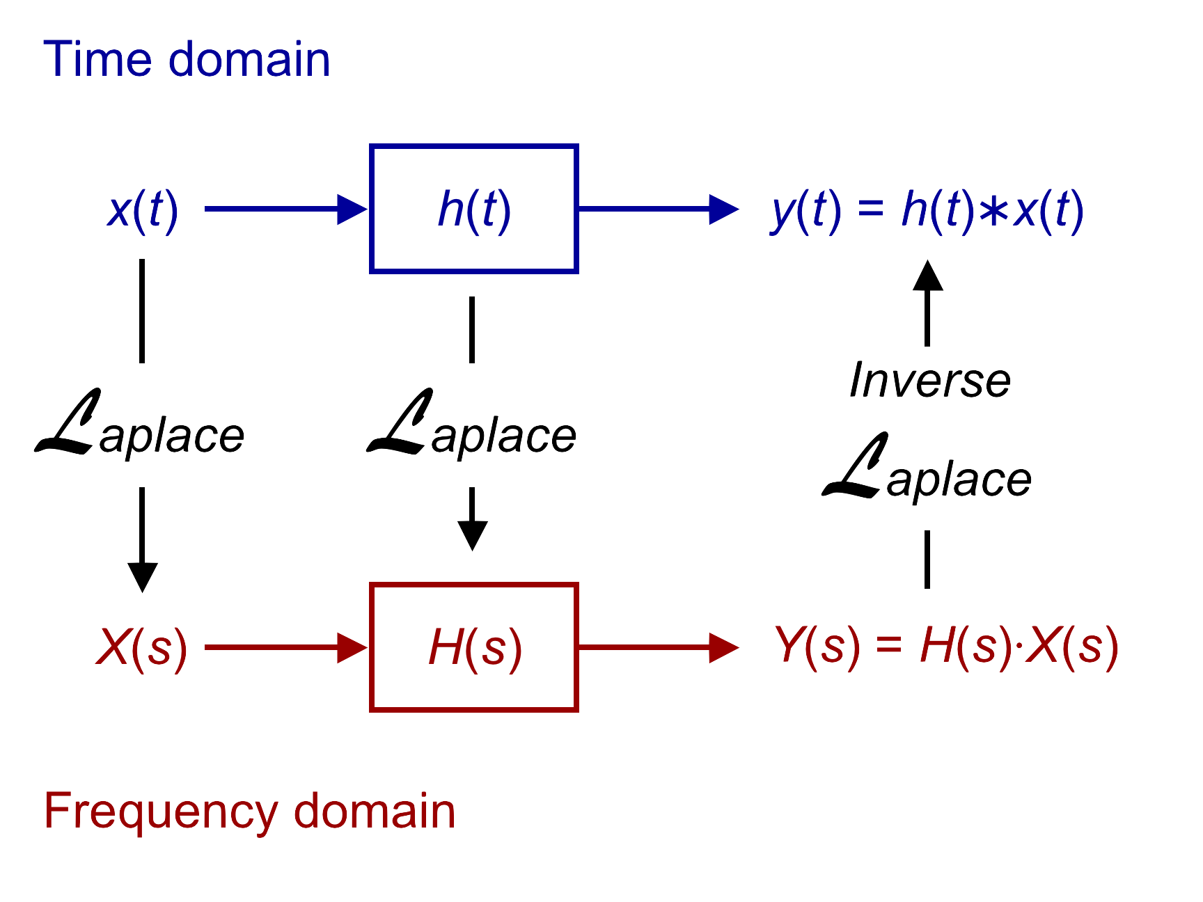
Commutative diagram: time-domain x(t), h(t), y(t)=h(t)*x(t) on top; Laplace transform down to frequency-domain X(s), H(s), Y(s)=H(s)X(s) on bottom; inverse Laplace back up
Figure 2.1.a. The Laplace transform turns the time-domain convolution \(y(t)=h(t)*x(t)\) into the frequency-domain product \(Y(s)=H(s)X(s)\) (Eq. (2.4)); the diagram commutes, so computing \(y(t)\) via \(H(s)X(s)\) then inverting is equivalent to convolving directly, and is almost always the easier route.

2.1.3  From LCCDE to transfer function

Apply the Laplace transform to the LCCDE, using the differentiation property \(\mathcal{L}\{d^rf/dt^r\} = s^rF(s) - s^{r-1}f(0^-) - \cdots - f^{(r-1)}(0^-)\). Assuming zero initial conditions (\(x^{(r)}(0^-)=y^{(r)}(0^-)=0\) for all \(r\), the standard assumption for system analysis) makes every initial-condition term vanish, converting the differential equation into a purely algebraic one:

$$\big(a_0+a_1s+\cdots+a_Ns^N\big)Y(s) = \big(b_0+b_1s+\cdots+b_Ms^M\big)X(s)$$
$$\boxed{H(s) = \frac{Y(s)}{X(s)} = \frac{b_0+b_1s+\cdots+b_Ms^M}{a_0+a_1s+\cdots+a_Ns^N} = K\,\frac{\prod_{k=1}^{M}(s-z_k)}{\prod_{\ell=1}^{N}(s-p_\ell)}.}$$
(2.5)

Factoring the numerator and denominator into roots exposes the zeros \(z_k\) (where \(H(s)=0\)) and poles \(p_\ell\) (where \(H(s)\to\infty\)); \(K\) is the overall gain. Zeros shape spectral notches; poles, as Section 2.4 shows, govern stability. A pole–zero plot (poles marked \(\times\), zeros marked \(\circ\), in the complex \(s\)-plane) is the single most useful sketch of a system, and is exactly the picture Lecture 5 draws over and over while designing filters.

MATLAB corner

MATLAB stores the numerator and denominator of Eq. (2.5) as two coefficient vectors. The tf() command turns them into a transfer-function model, and pole() and zero() find the roots for us. This is useful for checking hand calculations and for seeing stability directly on a pole–zero map.

Goal: build \(H(s)\) from the LCCDE's coefficients and read its poles/zeros straight off the object, instead of factoring by hand.
tf_from_lccde.m
MATLAB
% tf_from_lccde.m - transfer function from LCCDE, worked example with
% complex-conjugate poles (Eq. 2.5, Examples 2.6 and 2.7)
num = [5 25]; den = [1 4 29];
H = tf(num,den);
disp('H(s) ='); disp(H)
p = pole(H); z = zero(H); disp('Poles:'); disp(p); disp('Zeros:'); disp(z)
pzmap(H); grid on; hold on
hp = plot(real(p), imag(p), 'rx', 'MarkerSize',14, 'LineWidth',2); % poles
hz = plot(real(z), imag(z), 'go', 'MarkerSize',12, 'LineWidth',2); % zeros
ylim([-6 6])
legend([hp hz], {'Poles','Zeros'}, 'Location','best') % legend for markers
% Poles at Re(s) = -2 < 0 (open LHP) => system is stable
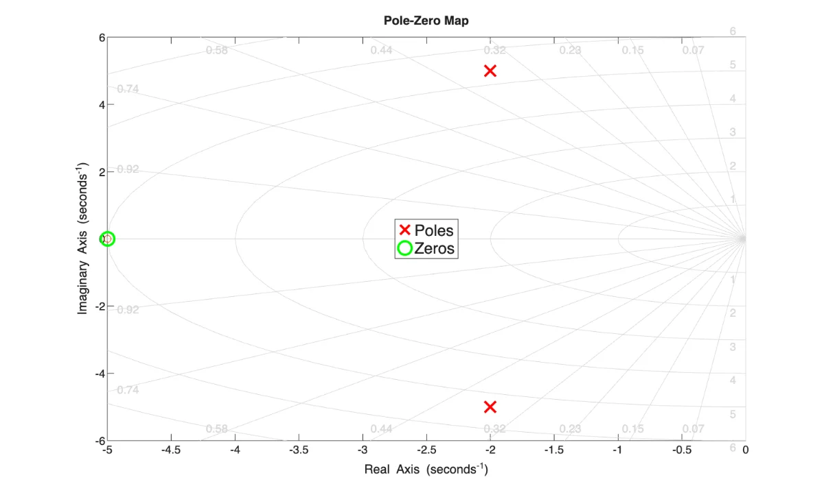
Figure 2.1.b — pole-zero map produced by tf_from_lccde.m
Figure 2.1.b. Reading the MATLAB pole–zero map. Crosses mark the poles at \(s=-2\pm j5\), and the circle marks the zero at \(s=-5\). Both poles have negative real part, so their time-domain terms contain the decaying factor \(e^{-2t}\). A causal system with these poles is therefore stable. The zero changes the gain and phase, but it does not decide stability; that decision comes from the pole locations.

2.2  The region of convergence: the half of the answer the algebra hides

A Laplace transform is more than an algebraic expression in \(s\). Its defining integral may converge for some values of \(s\) and diverge for others. The set of values for which it converges is the region of convergence (ROC). The pair “expression plus ROC” is needed to identify the time-domain signal uniquely.

The bilateral definition includes all time and therefore makes no assumption about what happened before \(t=0\):

$$F(s)=\int_{-\infty}^{\infty} f(t)\,e^{-st}\,dt, \qquad s=\sigma+j\Omega,$$
(2.6)

Because \(|e^{-st}|=e^{-\sigma t}\), convergence depends on \(\sigma=\operatorname{Re}\{s\}\), not on \(\Omega\). An ROC therefore appears as a vertical half-plane or strip in the \(s\)-plane. Its boundaries pass through poles, which are never included in the ROC.

2.2.1  Two signals, one algebraic expression

Transform the right-sided exponential \(f(t)=e^{-at}u(t)\). The integral runs from \(0\) to \(\infty\) and converges only when the integrand decays, i.e. when \(\sigma+a>0\):

$$e^{-at}u(t) \;\longleftrightarrow\; \frac{1}{s+a}, \qquad \text{ROC: } \sigma > -a.$$
(2.7)

Now transform the left-sided signal \(g(t)=-e^{-at}u(-t)\), which is zero for \(t>0\). The integral runs from \(-\infty\) to \(0\), and converges under the opposite condition:

$$-e^{-at}u(-t) \;\longleftrightarrow\; \frac{1}{s+a}, \qquad \text{ROC: } \sigma < -a.$$
(2.8)

Both signals produce the same expression, \(1/(s+a)\). The ROC tells us which signal is meant. An ROC to the right of the pole gives the right-sided, causal signal. An ROC to the left gives the left-sided, anti-causal signal. Lecture 4 uses the same idea for the \(z\)-transform.

σ s = −a ROC: σ > −a right-sided, causal f(t) = e −at u(t) σ s = −a ROC: σ < −a left-sided, anti-causal f(t) = −e −at u(−t)
Figure 2.2. Why the ROC is part of the answer. Both panels have the pole at \(s=-a\) and the expression \(F(s)=1/(s+a)\). In the left panel, convergence to the right of the pole produces a causal, right-sided exponential. In the right panel, convergence to the left produces an anti-causal, left-sided exponential. The shaded regions are vertical because convergence depends only on \(\operatorname{Re}\{s\}\). Neither region includes the pole.

Three ROC rules. First, an ROC never contains a pole. Second, a right-sided signal has an ROC to the right of its rightmost pole; a left-sided signal has an ROC to the left of its leftmost pole; and a two-sided signal has a strip between poles. Third, an absolutely integrable finite-duration signal has an ROC covering the whole \(s\)-plane.

EXAMPLE 2.1 · ROC decides the signal

A system has \(F(s)=\dfrac{1}{(s+1)(s-2)}\). Write down every signal \(f(t)\) consistent with this expression, and state which one is causal and which one is stable.

Step 1. Partial fractions give \(F(s)=\dfrac{-1/3}{s+1}+\dfrac{1/3}{s-2}\). The poles are at \(s=-1\) and \(s=+2\), so the plane is cut into three vertical strips, and each is a legitimate ROC.

Step 2. ROC \(\sigma>2\) (right of both poles): both terms are right-sided.

$$f(t) = \tfrac{1}{3}\big(e^{2t}-e^{-t}\big)u(t).$$

Step 3. ROC \(\sigma<-1\) (left of both poles): both terms are left-sided.

$$f(t) = \tfrac{1}{3}\big(e^{-t}-e^{2t}\big)u(-t).$$

Step 4. ROC \(-1<\sigma<2\) (the strip between them): the pole to the left contributes a right-sided term, the pole to the right a left-sided one.

$$f(t) = -\tfrac{1}{3}e^{-t}u(t) - \tfrac{1}{3}e^{2t}u(-t).$$

Step 5. The ROC \(\sigma>2\) is to the right of the rightmost pole, so its signal is causal. However, that ROC does not include the \(j\Omega\)-axis, so the signal is not stable. The middle strip \(-1<\sigma<2\) includes the \(j\Omega\)-axis, so it is stable, but it is two-sided and not causal. Because one pole lies in the right-half plane, no ROC can make this system both causal and stable.

2.2.2  Unilateral and bilateral: which one you are actually using

Many engineering problems begin at \(t=0\) and ask for the response afterwards. The unilateral Laplace transform is designed for this situation:

$$F(s)=\int_{0^-}^{\infty} f(t)\,e^{-st}\,dt.$$
(2.9)

The lower limit \(0^-\) includes an impulse at the origin, so \(\mathcal{L}\{\delta(t)\}=1\). A unilateral transform represents a right-sided signal, so its ROC is automatically to the right of the rightmost pole and is often omitted. Use the bilateral transform when behaviour before \(t=0\) matters or when the signal is two-sided.

The main advantage of the unilateral form is that it includes initial conditions directly. Its differentiation rules allow differential equations with a nonzero starting state to be solved algebraically:

$$\mathcal{L}\left\{\frac{df}{dt}\right\} = sF(s)-f(0^-), \qquad \mathcal{L}\left\{\frac{d^2f}{dt^2}\right\} = s^2F(s)-sf(0^-)-f'(0^-).$$
(2.10)

2.2.3  Initial and final value theorems

The initial and final values of a signal can sometimes be found directly from \(F(s)\), without calculating the full inverse transform:

$$f(0^+) = \lim_{s\to\infty} sF(s), \qquad \lim_{t\to\infty} f(t) = \lim_{s\to 0} sF(s).$$
(2.11)

For a strictly proper rational \(F(s)\), the initial value theorem is straightforward to use. The final value theorem requires an extra check: every pole of \(sF(s)\) must lie strictly in the left-half plane. Otherwise, the signal grows or continues to oscillate and has no final value. Always check the poles before using the second limit.

EXAMPLE 2.2 · Final value, applied and misapplied

For the step response of a stable first-order system, \(F(s)=\dfrac{5}{s(s+2)}\), find \(f(0^+)\) and \(f(\infty)\). Then try the same on \(G(s)=\dfrac{5}{s(s^2+9)}\) and say what goes wrong.

Step 1. Initial value: \(sF(s)=\dfrac{5}{s+2}\to 0\) as \(s\to\infty\), so \(f(0^+)=0\). The step response starts from rest, as it must.

Step 2. Final value: the poles of \(sF(s)=5/(s+2)\) are at \(s=-2\), strictly in the left-half plane, so the theorem applies:

$$\lim_{t\to\infty} f(t) = \lim_{s\to0}\frac{5}{s+2} = 2.5.$$

Inverting confirms it: \(f(t)=2.5\,(1-e^{-2t})u(t)\), which settles at \(2.5\).

Step 3. Now \(G(s)\). Mechanically, \(sG(s)=\dfrac{5}{s^2+9}\to 5/9\) as \(s\to0\) — an answer, and a plausible-looking one.

Step 4. But \(sG(s)\) has poles at \(s=\pm j3\), on the \(j\Omega\)-axis, not strictly left of it. Inverting gives \(g(t)=\tfrac{5}{9}\big(1-\cos 3t\big)u(t)\), which oscillates forever between \(0\) and \(10/9\) and has no limit. The theorem's precondition failed, so its output was meaningless. Always check the poles of \(sF(s)\) before quoting a final value.

2.3  Partial fractions: inverting the Laplace transform

Most transfer functions are ratios of polynomials in \(s\). Direct inversion may be difficult, so we first split the expression into simpler fractions. Each simple term then matches a standard Laplace-transform pair.

Distinct real poles. If \(F(s)=P(s)/Q(s)\) has \(N\) distinct poles \(p_1,\ldots,p_N\),

$$F(s) = \sum_{k=1}^{N}\frac{A_k}{s-p_k} \quad\Longrightarrow\quad f(t) = \sum_{k=1}^{N} A_k\,e^{p_kt}\,u(t).$$
(2.12)

Each pole \(p_k\) contributes one exponential term \(e^{p_kt}\): this is the key idea behind the whole method. Repeated poles use the table pair below, one term per power of the repeated factor:

$$ \mathcal{L}^{-1}\{1/(s+a)^n\} = \frac{t^{n-1}}{(n-1)!}e^{-at}u(t). $$
(2.13)
EXAMPLE 2.3 · Distinct real poles

Find \(f(t)=\mathcal{L}^{-1}\{F(s)\}\) for \(F(s) = \dfrac{4s+8}{s^2+5s+6}\).

Step 1. Factor: \(s^2+5s+6=(s+2)(s+3)\). Write \(F(s)=\dfrac{A}{s+2}+\dfrac{B}{s+3}\), so \(4s+8=A(s+3)+B(s+2)\).

Step 2. At \(s=-2\): \(0=A(1)\Rightarrow A=0\). At \(s=-3\): \(-4=B(-1)\Rightarrow B=4\).

$$F(s)=\frac{4}{s+3} \quad\Longrightarrow\quad \boxed{f(t)=4e^{-3t}u(t).}$$
EXAMPLE 2.4 · Repeated pole

Find \(f(t)\) for \(F(s)=\dfrac{3}{(s+1)^2}\).

Solution. Direct table lookup, \(\mathcal{L}^{-1}\{1/(s+a)^n\}=\frac{t^{n-1}}{(n-1)!}e^{-at}u(t)\) with \(n=2,a=1\):

$$\boxed{f(t) = 3t\,e^{-t}u(t).}$$
EXAMPLE 2.5 · Higher-order repeated pole

Find \(f(t)\) for \(F(s)=\dfrac{2s+5}{(s+2)^3}\).

Solution. Expand \(F(s)=\dfrac{A}{s+2}+\dfrac{B}{(s+2)^2}+\dfrac{C}{(s+2)^3}\); solving gives \(A=0,\ B=2,\ C=1\), so \(F(s)=\dfrac{2}{(s+2)^2}+\dfrac{1}{(s+2)^3}\). Inverting each term:

$$\boxed{f(t) = e^{-2t}\Big(2t+\tfrac{t^2}{2}\Big)u(t).}$$

2.3.1  Complex-conjugate poles

A complex-conjugate pole pair \(p_{1,2}=-\alpha\pm j\beta\) produces an oscillatory response. This occurs frequently in circuits, mechanical systems and control loops. A corresponding second-order term has the form \(H(s)=\dfrac{As+B}{(s+\alpha)^2+\beta^2}\). Two standard transform pairs are enough to invert it:

$$\mathcal{L}^{-1}\!\left\{\frac{s+\alpha}{(s+\alpha)^2+\beta^2}\right\} = e^{-\alpha t}\cos(\beta t), \qquad \mathcal{L}^{-1}\!\left\{\frac{\beta}{(s+\alpha)^2+\beta^2}\right\} = e^{-\alpha t}\sin(\beta t).$$
(2.14)

Step 1. Rewrite the numerator as a combination of \((s+\alpha)\) and \(\beta\): \(As+B = A(s+\alpha) + (B-A\alpha)\); writing \(C=(B-A\alpha)/\beta\) gives \(As+B = A(s+\alpha)+C\beta\), so

$$H(s) = A\,\frac{s+\alpha}{(s+\alpha)^2+\beta^2} + C\,\frac{\beta}{(s+\alpha)^2+\beta^2}.$$

Step 2. Apply the two standard pairs term by term:

$$\boxed{h(t) = e^{-\alpha t}\big[A\cos(\beta t)+C\sin(\beta t)\big]u(t) = D\,e^{-\alpha t}\sin(\beta t+\psi)\,u(t),}$$
(2.15)

where the amplitude–phase form uses \(D=\sqrt{A^2+C^2}\) and \(\tan\psi = A/C\) (both forms decay at the same rate \(e^{-\alpha t}\), only the bookkeeping differs).

EXAMPLE 2.6 · Complex-conjugate poles

Find \(f(t)\) for \(F(s) = \dfrac{5s+25}{s^2+4s+29}\).

Step 1. Complete the square: \(s^2+4s+29=(s+2)^2+25\), so \(\alpha=2,\ \beta=5\). Write the numerator as \(5s+25 = 5(s+2)+15\), so

$$F(s) = 5\,\frac{s+2}{(s+2)^2+25} + 15\,\frac{1}{(s+2)^2+25} = 5\,\frac{s+2}{(s+2)^2+25} + 3\,\frac{5}{(s+2)^2+25},$$

Step 2. matching the standard pairs with \(A=5\) and \(C=3\) (not \(15\): the second term's coefficient must be re-expressed in units of \(\beta=5\) before the pair applies). Then:

$$f(t) = e^{-2t}\big[5\cos(5t) + 3\sin(5t)\big]u(t).$$

Step 3. Combine the sine and cosine into one sinusoid. Expand \(R\sin(\beta t+\phi)\) and match coefficients with \(A\cos\beta t+C\sin\beta t\). This gives \(R\sin\phi=A=5\) and \(R\cos\phi=C=3\). Therefore:

$$R=\sqrt{A^2+C^2}=\sqrt{34}=5.83, \qquad \phi=\arctan\!\frac{A}{C}=\arctan\!\frac{5}{3}=1.03\ \text{rad},$$
$$\boxed{f(t) = e^{-2t}\big[5\cos(5t) + 3\sin(5t)\big]u(t) = 5.83\,e^{-2t}\sin(5t+1.03)\,u(t).}$$

The denominator is already in completed-square form, so the poles are \(s=-2\pm j5\). The imaginary part, \(5\), sets the oscillation frequency. The real part, \(-2\), produces the decaying envelope \(e^{-2t}\). Since both poles are in the open left-half plane, the causal system is stable.

MATLAB corner

Eq. (2.15) is the decaying oscillation \(h(t)\); its two exponential envelopes \(\pm\sqrt{A^2+C^2}\,e^{-\alpha t}\) pinch it at every peak, since \(\alpha\) alone sets the decay rate regardless of \(\beta\).

Goal: plot the actual decaying oscillation \(h(t)\) against its \(\pm e^{-\alpha t}\) envelope, to see the decay rate is set by \(\alpha\) alone.

damped_sinusoid_demo.m
MATLAB
% damped_sinusoid_demo.m - h(t) for complex-conjugate poles, Eq. (2.15)
% H(s) = (5s+25)/(s^2+4s+29): alpha=2, beta=5, A=5, C=3 (Examples 2.6 and 2.7)
alpha = 2; beta = 5; A = 5; C = 3;
t = 0:0.001:3;
h = exp(-alpha*t).*(A*cos(beta*t) + C*sin(beta*t)); % Eq. (2.15)
 
env = sqrt(A^2+C^2)*exp(-alpha*t); % +-e^(-alpha t) envelope
 
figure('Color','w'); hold on; grid on;
plot(t, h, 'LineWidth', 1.6);
plot(t, env, 'r--', t, -env, 'r--', 'LineWidth', 1.2);
xlabel('t (s)'); ylabel('h(t)');
legend('h(t) = e^{-2t}[5cos(5t)+3sin(5t)]', 'envelope \pm\surd(A^2+C^2)e^{-\alpha t}');
title('Damped oscillation decays inside its envelope, rate set by \alpha only');
 
% Sanity check against ilaplace, symbolically
syms s tt
Hs = (5*s+25)/(s^2+4*s+29);
ht = ilaplace(Hs, s, tt);
disp('Symbolic check via ilaplace:'); disp(simplify(ht))
Plot of h(t) = e^(-2t)[5cos(5t)+3sin(5t)] as a decaying oscillation, overlaid with its plus and minus envelope curves sqrt(A^2+C^2) e^(-alpha t), which pinch the oscillation at every peak and decay to zero by about t=2.5 seconds.
Figure 2.3. What the MATLAB result shows. The response \(h(t)=e^{-2t}[5\cos(5t)+3\sin(5t)]\) oscillates between the two envelope curves \(\pm\sqrt{5^2+3^2}\,e^{-2t}\). The imaginary part of the poles, \(\beta=5\), sets the oscillation rate. The real part, \(-\alpha=-2\), sets how quickly the envelope decays. Changing \(\beta\) would move the peaks closer together or farther apart; it would not change the decay rate.

2.4  Stability

Impulse response

Stable if \(h(t)\to0\) (or a finite value) as \(t\to\infty\).

BIBO

Every bounded input, \(|x(t)|\le M_x<\infty\), gives a bounded output, \(|y(t)|\le M_y<\infty\).

Asymptotic

Bounded initial conditions produce outputs that decay to zero as \(t\to\infty\).

Marginally stable

Simple poles sit on the \(j\Omega\)-axis, none to its right: \(h(t)\) neither decays nor grows. BIBO still fails — a matching input resonates it unboundedly.

All three reduce to one geometric test on the pole–zero plot: for a causal system, every pole must lie in the open left-half \(s\)-plane,

$$ \Re\{p_k\} < 0 \quad \forall k. $$
(2.16)

A pole on or to the right of the \(j\Omega\)-axis means \(h(t)\) does not decay, and BIBO stability fails.

STABLE (LHP) UNSTABLE (RHP) Re{s} Im{s} MARGINAL
Figure 2.4.a. Poles anywhere in the shaded left-half plane give a stable system; the right-half plane is unstable, and the orange jΩ-axis itself is the marginally stable boundary.
real pole, LHP → decays real pole, RHP → grows pole at origin → marginal complex pair, LHP → damped complex pair, RHP → grows pair on jΩ-axis → marginal
Figure 2.4.b. How pole position changes the response. A pole in the left half-plane produces a mode that decays with time, while a pole in the right half-plane produces a growing mode and therefore instability. A pole exactly on the \(j\Omega\)-axis produces an oscillation that does not decay; this is the marginal case. The horizontal position controls growth or decay, and the vertical position controls oscillation frequency.

2.4.1  Reading stability off a complex pole pair

For the important case \(p_{1,2}=-\alpha\pm j\beta\), the impulse response has the form \(h(t)=D e^{-\alpha t}\sin(\beta t+\phi)u(t)\). The two parts of each pole have different roles: \(\beta\) sets the oscillation frequency, while \(-\alpha\) determines whether the envelope decays, remains constant or grows.

Real part \(-\alpha\) · the envelope

Sets the exponent of \(e^{-\alpha t}\): how fast the response dies, or whether it dies at all. Distance from the \(j\Omega\)-axis is the decay rate.

Imaginary part \(\beta\) · the ripple

Sets the frequency of \(\sin(\beta t+\phi)\): how fast it rings. Height above the real axis is the oscillation frequency. It has no say in stability.

So stability is decided by the sign of \(\alpha\) alone, and there are exactly three outcomes:
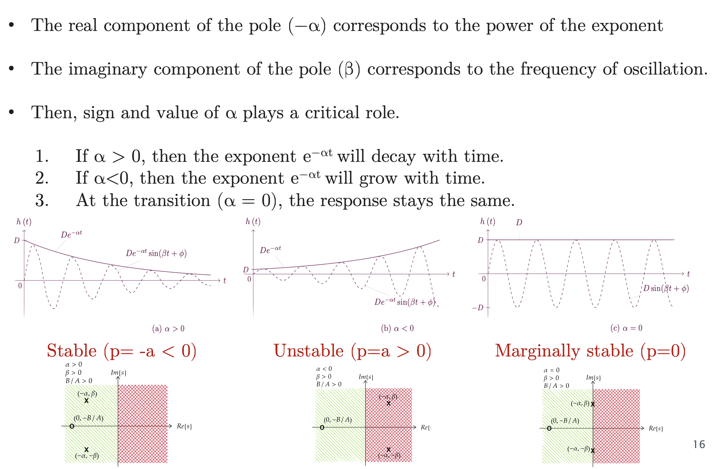
Three columns comparing a complex conjugate pole pair: alpha greater than zero gives a decaying envelope and a stable pole pair in the left half plane; alpha less than zero gives a growing envelope and an unstable pair in the right half plane; alpha equal to zero gives a constant-amplitude oscillation with the pair on the imaginary axis
Figure 2.4.c. One pole pair, three fates. The dashed curve is \(h(t)\), the solid curve its envelope \(D e^{-\alpha t}\). (a) \(\alpha>0\): the pair sits in the left half-plane, the envelope decays, the system is stable. (b) \(\alpha<0\): the pair has crossed into the right half-plane and the same oscillation grows without bound, unstable. (c) \(\alpha=0\): the pair sits exactly on the \(j\Omega\)-axis, the envelope is flat, and the system rings forever at \(\beta\) — marginally stable. Note the ringing frequency \(\beta\) is identical in all three; only the horizontal position of the poles changed.

Marginal stability is a boundary case, not a comfortably stable one. Poles on the \(j\Omega\)-axis produce oscillations that do not decay. A bounded input at the same frequency can make the response grow through resonance, so BIBO stability fails. An ideal lossless \(LC\) circuit would behave this way. In a real \(RLC\) circuit, resistance moves the poles into the left-half plane and gives the resonance a finite height.
EXAMPLE 2.7 · Capstone: LCCDE → transfer function → stability → h(t)

A system obeys \(y''(t)+4y'(t)+29y(t) = 5x'(t)+25x(t)\). Find \(H(s)\), classify its stability, and find \(h(t)\).

Step 1. Laplace-transform both sides under zero initial conditions (Section 2.1.3): \((s^2+4s+29)Y(s) = (5s+25)X(s)\), so

$$H(s) = \frac{Y(s)}{X(s)} = \frac{5s+25}{s^2+4s+29}.$$

Step 2. Poles: \(s^2+4s+29=0 \Rightarrow s = \dfrac{-4\pm\sqrt{16-116}}{2} = -2\pm j5\). Both poles satisfy \(\Re\{s\}=-2<0\): the system is BIBO stable (Section 2.4).

Step 3. Its impulse response is exactly Example 2.6's result,

$$\boxed{h(t) = e^{-2t}\big[5\cos(5t)+3\sin(5t)\big]u(t),}$$

a damped oscillation, as the pole picture in Section 2.4 predicts. Because the system is stable, its region of convergence includes the \(j\Omega\)-axis, so \(H(j\Omega)\) (the object every later filter-design lecture shapes on purpose) is well defined (Section 2.6).

EXAMPLE 2.8 · An unstable system, from h(t) to the step response

A system has \(h(t)=\tfrac12 e^{-t}\big(e^{2t}-1\big)\). Find \(H(s)\), locate its poles, classify it, and find the unit-step response.

Step 1. Expanding first is the whole trick: \(h(t)=\tfrac12 e^{t}-\tfrac12 e^{-t}\), which is a sum of two exponentials, so Section 2.3 runs backwards and each term contributes one pole:

$$H(s)=\frac{1}{2(s-1)}-\frac{1}{2(s+1)}=\frac{1}{(s-1)(s+1)}.$$

Step 2. The poles are \(p=\pm1\). One of them, \(p=+1\), lies in the right half-plane, so Eq. (2.16) fails and the system is unstable — and the \(e^{+t}\) term in \(h(t)\) says so directly.

Step 3 · Step response. With \(x(t)=u(t)\), \(X(s)=1/s\), so \(Y(s)=H(s)/s\). Partial fractions on the three distinct poles \(\{0,+1,-1\}\) give

$$Y(s)=\frac{1}{2(s-1)}-\frac{1}{s}+\frac{1}{2(s+1)} \ \xrightarrow{\ \mathcal{L}^{-1}\ }\ \boxed{y(t)=-1+\tfrac12 e^{-t}+\tfrac12 e^{t}.}$$

The step input is bounded, but the output grows without limit because of the \(e^t\) term. The system therefore fails the BIBO stability test. The pole at \(+1\) predicted this result directly. No ROC for this causal system includes the \(j\Omega\)-axis, so a conventional frequency response \(H(j\Omega)\) does not exist.

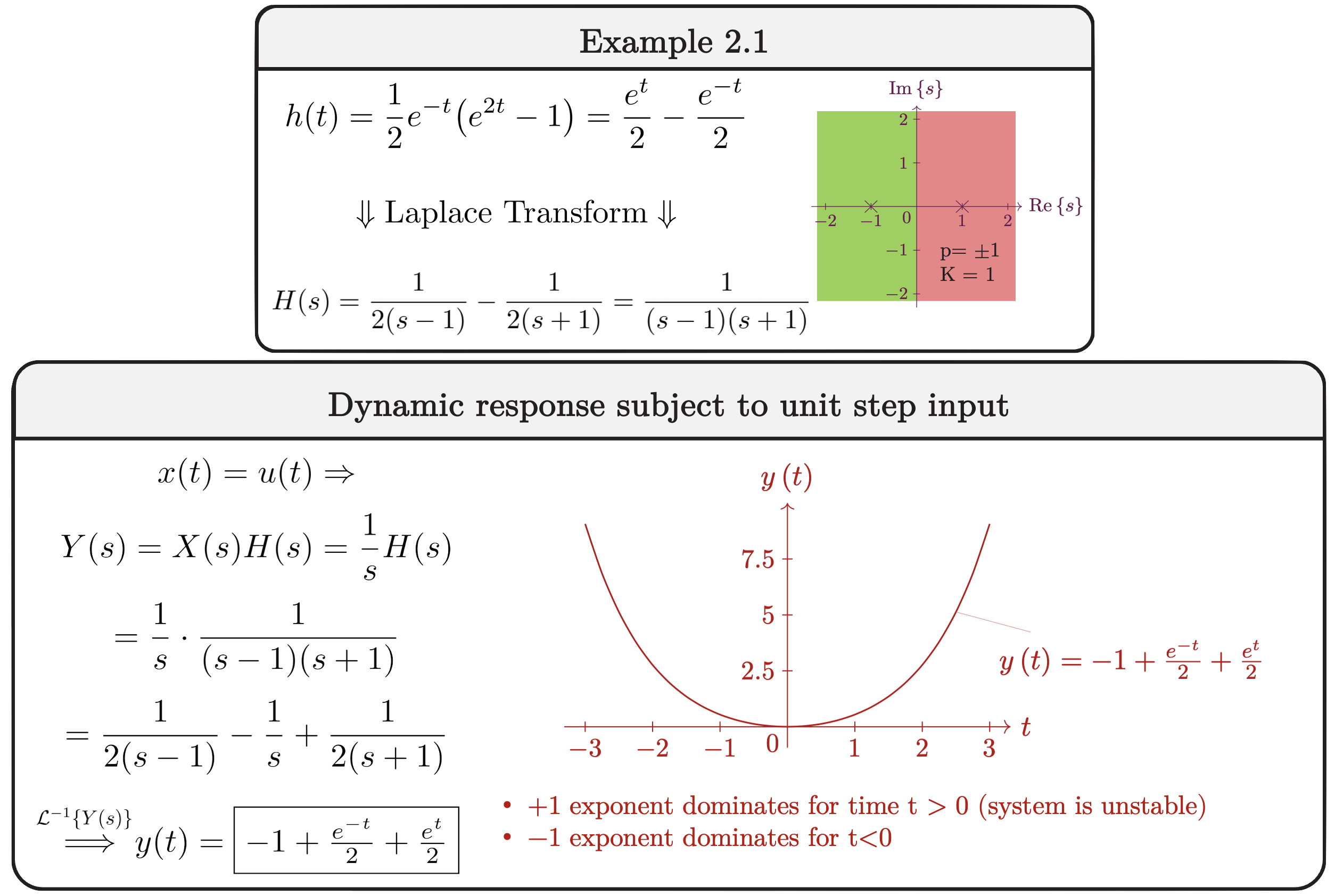
Worked example: h(t) = half e to the minus t times (e to the 2t minus 1) transformed to H(s) = 1/((s-1)(s+1)) with poles marked at plus and minus one on a pole-zero plot, and below, the unit step response y(t) = -1 + e^-t/2 + e^t/2 growing without bound

How to read the result. The upper plots connect the impulse response with its poles. The pole at \(+1\) lies in the unstable half-plane and creates a growing exponential. The lower plot shows the consequence: a bounded step input produces an unbounded output. This confirms the pole test without needing to inspect every time-domain term.

MATLAB corner

MATLAB can apply the stability test in Eq. (2.16) directly: find the poles and inspect the signs of their real parts. The pzmap() command then makes the comparison visual. Poles in the left half-plane produce decaying modes; any pole in the right half-plane produces a growing mode.

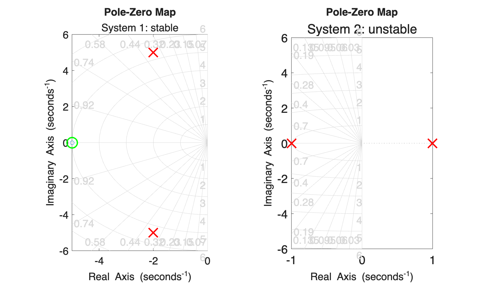
Goal: verify the RHP/LHP stability test numerically on both a stable and an unstable system, and reproduce Figure 2.3 from real pole-zero maps.
pole_zero_stability_check.m
MATLAB
% compare_systems_pz.m - increase font and emphasize poles/zeros
sys(1).num = [5 25]; sys(1).den = [1 4 29];
sys(2).num = [1]; sys(2).den = [1 0 -1];
figure('Color','w');
for k = 1:2
   p = roots(sys(k).den);
   stable = all(real(p) < 0);
   fprintf('System %d poles: %s -> stable: %d\n', k, mat2str(p,3), stable);
   ax = subplot(1,2,k);
   H = tf(sys(k).num, sys(k).den);
   pzmap(H); grid on; hold on
   plot(real(p), imag(p), 'rx', 'MarkerSize',20, 'LineWidth',2); % emphasize poles
   z = zero(H);
   fontsize(gcf,16,"points") % increase all figure font sizes
   plot(real(z), imag(z), 'go', 'MarkerSize',16, 'LineWidth',2); % emphasize zeros
   ylim(ax,[-6 6])
   ax.FontSize = 18;
   if stable
      title(ax,'System ' + string(k) + ': stable');
   else
      title(ax,'System ' + string(k) + ': unstable');
   end
end
Two pole-zero maps side by side: System 1 (stable) has a complex-conjugate pole pair at -2+-5j marked with red x's, in the left half-plane, with a zero circle at -5; System 2 (unstable) has poles at +1 and -1 marked with red x's, one pole in the right half-plane
Figure 2.4.d. Comparing the two MATLAB results. The system from Examples 2.6 and 2.7 has poles at \(-2\pm j5\). Both are in the left half-plane, so every natural mode decays and the causal system is stable. Example 2.8 has poles at \(-1\) and \(+1\). The pole at \(+1\) creates an \(e^t\) term that grows without bound, so the system is unstable. One right-half-plane pole is enough to fail the stability test, even if every other pole is stable.

2.5  Reading a system off its pole-zero plot

A pole-zero plot collects several important properties in one picture. It shows natural modes, stability and the main features of the frequency response. For this reason, it is often the first plot used to inspect a system and the final plot checked after a design.

A rational transfer function is fixed, up to a gain, by where its poles and zeros sit:

$$H(s) = K\,\frac{\prod_{k=1}^{M}(s-z_k)}{\prod_{\ell=1}^{N}(s-p_\ell)}.$$

At a chosen value of \(s\), each factor represents the distance from a pole or zero to that point. On the \(j\Omega\)-axis, the magnitude tends to increase near a pole and decrease near a zero. This geometric rule helps predict resonances and attenuation directly from the plot and becomes a central design idea in Lecture 5.

QuestionWhat to look atAnswer
Stable?Does the ROC contain the \(j\Omega\)-axis?Yes ⇒ BIBO stable. For a causal system this reduces to: all poles strictly in the left-half plane.
Causal?Is the ROC right of the rightmost pole?Yes ⇒ causal. The poles alone cannot tell you; the ROC can.
Both at once?Rightmost pole.Possible only if every pole is in the left-half plane.
Invertible by a stable causal system?Zeros.Only if every zero is also in the left-half plane — a minimum-phase system.
How fast does it settle?Distance of the dominant pole from the \(j\Omega\)-axis.Time constant \(1/|\sigma|\); the pole nearest the axis dominates.

2.5.1  Invertibility, and why zeros have a side too

Inverting a system means undoing it: finding \(H_{\mathrm{inv}}(s)\) such that the cascade is the identity. Algebraically this is trivial —

$$H_{\mathrm{inv}}(s)=\frac{1}{H(s)}=\frac{1}{K}\,\frac{\prod_{\ell}(s-p_\ell)}{\prod_{k}(s-z_k)},$$
(2.17)

The zeros of \(H\) become the poles of the inverse \(H_{\mathrm{inv}}\). Therefore, a right-half-plane zero in the original system becomes an unstable pole in its causal inverse. A stable causal system whose poles and zeros are all in the left-half plane is called minimum phase. Such a system can have a stable causal inverse.

σ pole −2 zero −1 MINIMUM PHASE inverse (s+2)/(s+1) is stable and causal σ pole −2 zero +1 NON-MINIMUM PHASE inverse (s+2)/(s−1) is unstable
Figure 2.5. Two systems with the same poles and the same magnitude response. Only the left one is minimum phase; mirroring its zero across the \(j\Omega\)-axis leaves \(|H(j\Omega)|\) unchanged but makes the inverse unstable.

The name comes from a second fact: among all systems sharing one magnitude response, the minimum-phase one has the least phase lag and the fastest energy build-up. Any other is that system cascaded with an all-pass factor,

$$H(s) = H_{\min}(s)\cdot \underbrace{\frac{s-a}{s+a}}_{\text{all-pass}}, \qquad \left|\frac{j\Omega-a}{j\Omega+a}\right| = 1 \;\; \text{for all } \Omega,$$
(2.18)

which changes the phase while leaving the magnitude untouched. This is why a magnitude specification alone never pins down a filter, and why Lecture 5's design methods must say something about phase separately.

EXAMPLE 2.9 · Which of these can be equalised?

A communications channel is modelled as \(H_1(s)=\dfrac{s-4}{(s+1)(s+3)}\); a second channel as \(H_2(s)=\dfrac{s+4}{(s+1)(s+3)}\). Both are causal. Which can be equalised by a stable causal filter, and what do they have in common?

Step 1. Both have poles at \(s=-1,-3\), strictly in the left-half plane, so both are stable and causal.

Step 2. Their zeros differ: \(H_1\) has a zero at \(s=+4\) (right-half plane), \(H_2\) at \(s=-4\) (left-half plane). Only \(H_2\) is minimum phase.

Step 3. The equaliser for \(H_2\) is \(1/H_2(s)=\dfrac{(s+1)(s+3)}{s+4}\): its pole is at \(s=-4\), so it is stable and causal. Usable.

Step 4. The equaliser for \(H_1\) would be \(\dfrac{(s+1)(s+3)}{s-4}\), with a pole at \(s=+4\). Stable or causal, not both — in practice, unusable.

Step 5. For every \(\Omega\), \(|j\Omega-4|=|j\Omega+4|\), so the two systems have identical magnitude responses. Their difference appears only in phase. A magnitude-only measurement therefore cannot reveal whether the zero is in the left- or right-half plane, and cannot determine whether a stable causal equalizer exists.

2.6  From Laplace to Fourier: the CTFT as a special case

Recall \(s=\sigma+j\Omega\), so the Laplace kernel splits into a damping factor and an oscillation: \(e^{-st}=e^{-\sigma t}e^{-j\Omega t}\). Setting \(\sigma=0\) strips away the damping and leaves a purely frequency-domain view:

$$\boxed{X(\Omega) = X(s)\big|_{s=j\Omega} = \int_{-\infty}^{\infty}x(t)\,e^{-j\Omega t}\,dt}$$
(2.19)

This is the Continuous-Time Fourier Transform (CTFT). It exists when the ROC of \(X(s)\) includes the \(j\Omega\)-axis. For a causal stable LTI system, all poles are in the left-half plane, so this condition is satisfied. Its frequency response is therefore obtained by evaluating the transfer function at \(s=j\Omega\).

ROC of X(s): σ > −2 σ = Re{s} jΩ-axis (σ = 0) p₁ = −2+j5 p₂ = −2−j5 0
Figure 2.6.a. Connecting stability and frequency response. For the causal system in Examples 2.6 and 2.7, the rightmost poles have real part \(-2\), so the ROC is \(\sigma>-2\). This region includes the \(j\Omega\)-axis at \(\sigma=0\), which means \(H(j\Omega)\) exists. If a causal system has a right-half-plane pole, its ROC begins to the right of that pole and no longer includes the axis; the ordinary frequency response then fails to exist.

The transform runs backwards through the same axis, giving the inverse CTFT, and, for a real-valued signal, the conjugate symmetry already met in Lecture 1 (Eq. 1.7):

$$\begin{aligned} x(t)&=\frac{1}{2\pi}\int_{-\infty}^{\infty} X(\Omega)\,e^{j\Omega t}\,d\Omega,\\[2pt] X(-\Omega)&=X^{*}(\Omega)\quad\text{for real }x(t). \end{aligned}$$
(2.20)

The analysis integral measures the amplitude and phase associated with each frequency. The synthesis integral adds those frequency components to reconstruct the signal. Because the transform is reversible, we can specify and design a system through its frequency response \(H(j\Omega)\), then return to the time domain when needed.

Three kernels, one idea, different amounts of damping

Every transform in this module probes a signal with an exponential and asks “how much of this is in there?” They differ only in how much decay the probe is allowed to carry:

\(e^{-st}\)
Laplace — damping \(\sigma\) is free, so even growing signals converge. Answers does it blow up, and how fast does it settle?
\(e^{-j\Omega t}\)
Fourier — \(\sigma\) forced to \(0\), so the signal must converge unaided. Answers how much sits at each frequency?
\(z^{-n}\)
\(z\)-transform (Lecture 4) — the discrete-time Laplace, with \(z=re^{j\omega}\); \(r\) plays the role of \(\sigma\), and \(r=1\) recovers the DTFT.

Setting \(\sigma=0\) is therefore a trade: you give up the ability to analyse unstable systems, and in exchange you get a picture with a direct physical meaning, a spectrum.

Removing the Laplace damping factor makes convergence more restrictive. In particular, the ordinary CTFT integral does not converge for a nonzero periodic signal:

$$\begin{aligned} E=\int_{-\infty}^{\infty}\cos^{2}(\Omega_0 t)\,dt &= \infty\\[2pt] \Longrightarrow\quad \int_{-\infty}^{\infty}\cos(\Omega_0 t)\,e^{-j\Omega t}\,dt &\ \text{ does not converge} \end{aligned}$$
(2.21)

This matches the distinction from Lecture 1. The ordinary CTFT is naturally suited to energy signals, while a nonzero periodic signal is a power signal. Periodic signals therefore need the Fourier series description introduced in Section 2.11. Discrete-time signals require the corresponding DTFT and DTFS forms developed later.

EXAMPLE 2.10 · CTFT of a one-sided exponential: s → jΩ made concrete

Find the CTFT of \(x(t)=e^{-at}u(t)\), \(a>0\), and its magnitude and phase.

Solution. The step confines the integral to \(t\ge0\), and the combined exponent decays because \(a>0\):

$$\begin{aligned} X(\Omega)=\int_{0}^{\infty}\!\!e^{-at}e^{-j\Omega t}dt=\left[\frac{e^{-(a+j\Omega)t}}{-(a+j\Omega)}\right]_{0}^{\infty}=\boxed{\frac{1}{a+j\Omega}} \end{aligned}$$
$$|X(\Omega)|=\frac{1}{\sqrt{a^{2}+\Omega^{2}}}, \quad \angle X(\Omega)=-\arctan\!\frac{\Omega}{a}$$

Three observations tie this back to the lecture:

(i) This is exactly \(H(s)=1/(s+a)\), the Laplace transform of the same signal, evaluated at \(s=j\Omega\), which is Eq. (2.19) in one concrete case.

(ii) The single pole at \(s=-a\) is in the left half-plane, so the system is stable and the CTFT was guaranteed to exist.

(iii) \(|X|\) falls monotonically and reaches \(1/\sqrt2\) of its DC value at \(\Omega=a\): a first-order low-pass with \(-3\,\text{dB}\) at \(\Omega=a\), i.e. the \(RC\) network of Figure 1.4 with \(a=1/RC\).

MATLAB corner

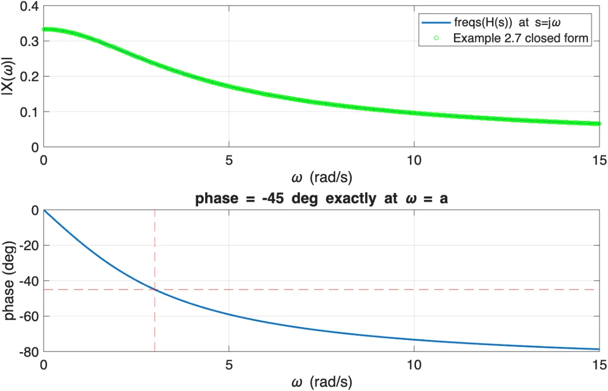
To obtain the frequency response, Eq. (2.19) evaluates the transfer function on the imaginary axis by setting \(s=j\Omega\). MATLAB's freqs() performs this calculation from the coefficient vectors. We compare its output with the closed-form expression from Example 2.10; the two should agree apart from numerical rounding.

Goal: evaluate \(H(s)=1/(s+a)\) at \(s=j\Omega\) via freqs() and confirm it matches Example 2.10's closed-form CTFT, including the \(-3\,\text{dB}\) point at \(\Omega=a\).
ctft_from_laplace.m
MATLAB
% ctft_from_laplace.m - Eq. (2.19): CTFT is H(s) evaluated at s = j*omega
a = 3; num = 1; den = [1 a]; % H(s) = 1/(s+a), Eq. (2.5) form
w = linspace(0, 15, 500);
 
Hjw = freqs(num, den, w); % MATLAB sets s = j*w for you - Eq. (2.19)
Hclosed = 1 ./ (a + 1j*w); % Example 2.10's closed-form answer
fprintf('max abs diff: %.2e\n', max(abs(Hjw - Hclosed)));
 
figure('Color','w');
subplot(2,1,1); plot(w,abs(Hjw),'LineWidth',1.8); hold on;
plot(w,abs(Hclosed),'go','MarkerSize',4); grid on;
legend('freqs(H(s)) at s=j\Omega', 'Example 2.10 closed form');
xlabel('\Omega (rad/s)'); ylabel('|X(\Omega)|');
 
subplot(2,1,2); plot(w, angle(Hjw)*180/pi, 'LineWidth', 1.8); grid on;
yline(-45,'r--'); xline(a,'r--');
xlabel('\Omega (rad/s)'); ylabel('phase (deg)');
title('phase = -45 deg exactly at \Omega = a');
Figure 2.6.b — magnitude and phase produced by ctft_from_laplace.m
Figure 2.6.b. Interpreting the MATLAB check. The samples returned by freqs() lie on the closed-form magnitude and phase curves, so evaluating \(H(s)\) at \(s=j\Omega\) gives the same frequency response as the direct CTFT calculation. At \(\Omega=a\), the magnitude has fallen to \(1/\sqrt{2}\) of its DC value, or \(-3\,\text{dB}\), and the phase is \(-45^\circ\). These two markers provide an easy numerical check of the result.

2.6.1  Convergence: when does the CTFT actually exist?

The substitution \(s=j\Omega\) is valid only when the \(j\Omega\)-axis lies inside the ROC. If it does not, the Fourier integral diverges. Two common sufficient conditions help us decide when a CTFT exists.

The first is absolute integrability, which guarantees the integral converges for every \(\Omega\):

$$\int_{-\infty}^{\infty} |x(t)|\,dt < \infty.$$
(2.22)

Together with the requirement that a finite interval contains only finitely many extrema and finite jumps, these form the Dirichlet conditions. At a continuous point, the inverse transform returns \(x(t)\). At a jump, it returns the midpoint of the two limiting values. Finite-energy signals may also converge in the mean-square sense, where the total error energy tends to zero even if individual points do not match exactly.

The sinc function decays as \(1/t\). It is square-integrable but not absolutely integrable, so its transform is interpreted through mean-square convergence. This issue appears again in the ideal brick-wall filter. Pure sinusoids and steps do not satisfy either ordinary condition; their Fourier transforms are represented using impulses in frequency. These impulse-valued transforms are useful, but they are generalized functions rather than ordinary curves.

2.7  Why complex exponentials? The basis an LTI system cannot break

Many sets of functions could be used to build a signal. Fourier analysis uses sinusoids, written compactly as complex exponentials, because they interact with LTI systems in an exceptionally simple way.

2.7.1  Sinusoids are the one shape an LTI system cannot change

Convolution adds scaled and delayed copies of the input. Delaying a sinusoid changes its phase but not its frequency. Adding several sinusoids at the same frequency produces another sinusoid at that frequency. Therefore, an LTI system can change a sinusoid's amplitude and phase, but not its frequency:

$$ A_1\sin(\Omega t+\varphi_1)+A_2\sin(\Omega t+\varphi_2) = A\sin(\Omega t+\varphi). $$
(2.23)
A₁ A₂ A three arrows, one angular speed Ω height of the sum = A·sin(Ωt + φ)
Figure 2.7.a. Why Eq. (2.23) is obvious once you look at it properly. Read \(A\sin(\Omega t+\varphi)\) as the height of an arrow of length \(A\) turning at \(\Omega\) rad/s from a start angle \(\varphi\). Two such arrows, turning at the same rate, stay rigidly locked to one another, so their tip-to-tail sum is a third arrow turning at that same rate. Amplitudes and phases change; the frequency cannot.

For example, a \(1\,\text{kHz}\) input to an LTI system produces a \(1\,\text{kHz}\) output. The output may be weaker, stronger or phase shifted, but it cannot become a different frequency or a square wave. A nonlinear system can create new frequencies; that behaviour is harmonic or intermodulation distortion.

2.7.2  Sinusoids of different frequencies are orthogonal

Closure alone would be useless if the components interfered with each other's bookkeeping. They do not: over a common period, distinct harmonics integrate against each other to exactly zero.

$$\begin{aligned} \int_{0}^{T_0}\!\cos(m\Omega_0t)\cos(n\Omega_0t)\,dt &= 0 \quad (m\neq n),\\[2pt] \int_{0}^{T_0}\!\sin(m\Omega_0t)\cos(n\Omega_0t)\,dt &= 0 \quad \forall m,n. \end{aligned}$$
(2.24)
sin(t) sin(2t) product sin(t)·sin(2t): shaded area above = shaded area below ⇒ integral = 0 0
Figure 2.7.b. Orthogonality is a cancellation, not a coincidence. The product of two different harmonics spends exactly as much area above the axis as below it over one common period, so the integral vanishes. Multiply a signal by \(e^{-jk\Omega_0t}\) and integrate, and every harmonic except the \(k\)th self-destructs, leaving that one coefficient behind.

Different complex exponentials are orthogonal, so each Fourier coefficient can be measured independently. Multiply the signal by the conjugate of the required basis function, then integrate or sum. The formulas for \(X(\Omega)\), \(X_k\), \(X(e^{j\omega})\) and \(X[k]\) all follow this same pattern.

2.7.3  Euler's formula: one object instead of two

Sines and cosines work, but they are clumsy: a sinusoid carries an amplitude and a phase, and keeping them in separate columns makes every calculation twice as long. Euler's identity collapses the pair.

$$\begin{aligned} e^{j\theta}&=\cos\theta+j\sin\theta\\[3pt] \Longleftrightarrow\quad \cos(\Omega t)&=\tfrac{1}{2}\big(e^{j\Omega t}+e^{-j\Omega t}\big), \qquad \sin(\Omega t)=\tfrac{1}{2j}\big(e^{j\Omega t}-e^{-j\Omega t}\big). \end{aligned}$$
(2.25)

Three concrete payoffs follow, and each one shows up somewhere later in the module.

  • Amplitude and phase become one number. The phasor \(Ae^{j\varphi}\) carries both, and complex multiplication applies a gain and a phase shift in one operation. That is exactly what a filter does to a tone, which is why a filter's whole effect at one frequency is the single complex number \(H(j\Omega)\).
  • Calculus becomes arithmetic. \(\frac{d}{dt}e^{j\Omega t}=j\Omega\,e^{j\Omega t}\) and \(\int e^{j\Omega t}dt = \frac{1}{j\Omega}e^{j\Omega t}\): differentiation is multiplication by \(j\Omega\), integration is division by it. This is the Fourier-domain echo of the \(s^k\) that appeared when the LCCDE was Laplace-transformed in Section 2.1.3.
  • Negative frequencies stop being mysterious. Eq. (2.25) says a real cosine is the sum of two counter-rotating phasors, one at \(+\Omega\) and one at \(-\Omega\). The negative half of every spectrum in this lecture is not a physical frequency; it is the other half of a real signal's conjugate pair, and it is why \(X(-\Omega)=X^{*}(\Omega)\).

2.7.4  The eigenfunction property: the reason the whole ladder exists

The three properties above converge on one statement. Push \(x[n]=e^{j\omega n}\) through the convolution sum of Eq. (1.14) and watch the exponential factor out:

$$ y[n]=\sum_{k=-\infty}^{\infty}h[k]\,e^{j\omega(n-k)} = e^{j\omega n}\underbrace{\sum_{k=-\infty}^{\infty}h[k]\,e^{-j\omega k}}_{\textstyle H(e^{j\omega}),\ \text{independent of }n}. $$
(2.26)

The output is the input multiplied by a constant. In the language of linear algebra, complex exponentials are the eigenfunctions of every LTI/LSI system, and the eigenvalue is the frequency response, exactly as Lecture 1's Problem 1.7 proved for \(z^n\):

$$\boxed{\;\begin{aligned} x(t)=e^{j\Omega t}\ &\Longrightarrow\ y(t)=H(j\Omega)\,e^{j\Omega t}\\[2pt] x[n]=e^{j\omega n}\ &\Longrightarrow\ y[n]=H(e^{j\omega})\,e^{j\omega n} \end{aligned}\;}$$
(2.27)

Now add linearity. If the input can be written as a sum of exponentials, the system acts on each one separately and never mixes them:

$$\begin{aligned} x(t)=\sum_k A_k e^{j\Omega_k t} \ &\xrightarrow{\ \text{LTI}\ }\ y(t)=\sum_k A_k\,H(j\Omega_k)\,e^{j\Omega_k t}\\[3pt] x[n]=\sum_k A_k e^{j\omega_k n} \ &\xrightarrow{\ \text{LSI}\ }\ y[n]=\sum_k A_k\,H(e^{j\omega_k})\,e^{j\omega_k n} \end{aligned}$$
(2.28)
MATLAB corner

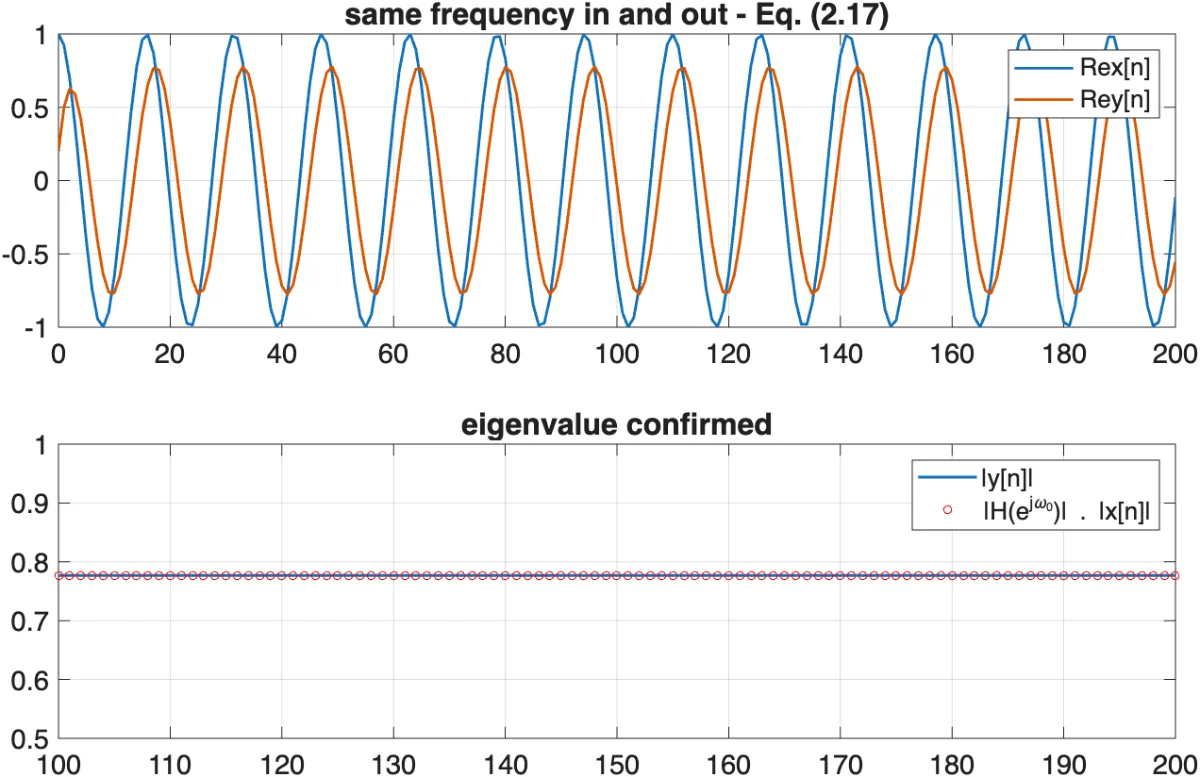
Eq. (2.26)–(2.27) are a strong claim: push a complex exponential through any LTI system and only a single complex number changes. That is easy to take on faith and easy to check.

Goal: filter a complex exponential through a real IIR system and verify the steady-state output is exactly the input multiplied by \(H(e^{j\omega_0})\).
eigenfunction_demo_fixed.m
MATLAB
% eigenfunction_demo_fixed.m - verify Eq. (2.26)-(2.27) numerically
b = [0.2 0.2]; a = [1 -0.6];
w0 = 0.4; % test frequency, rad/sample
n = (0:200)';
x = exp(1j*w0*n);
y = filter(b, a, x);
Hw0 = polyval(b, exp(-1j*w0)) ./ polyval(a, exp(-1j*w0)); % H(e^{j*w0}) evaluated directly
steady = 100:200;
predicted = Hw0 * x(steady+1);
fprintf('max steady-state error: %.2e\n', max(abs(y(steady+1) - predicted)));
figure('Color','w');
    fontsize(gcf,16,"points") % increase all figure font sizes
subplot(2,1,1); plot(n, real(x), n, real(y), 'LineWidth', 1.4); grid on;
legend('Re{x[n]}', 'Re{y[n]}'); title('same frequency in and out - Eq. (2.26)');
subplot(2,1,2);
plot(n(steady+1), abs(y(steady+1)), 'LineWidth',1.4); hold on;
plot(n(steady+1), abs(predicted), 'ro', 'MarkerSize',4); grid on;
ylim([0.5 1]); % set y-axis between 0.5 and 1
legend('|y[n]|', '|H(e^{j\omega_0})| . |x[n]|');
title('eigenvalue confirmed');
Figure 2.7.c — input/output overlay and steady-state amplitude match produced by eigenfunction_demo.m
Figure 2.7.c. What to notice in the MATLAB output. After the start-up transient has decayed, the output oscillates at exactly the same frequency as the complex-exponential input. Only its amplitude and phase have changed. Their measured values agree with \(|H(e^{j\omega_0})|\) and \(\angle H(e^{j\omega_0})\) to machine precision. This demonstrates why complex exponentials are eigenfunctions of LTI systems: the system changes their complex scale, not their frequency.
The one-sentence reason for everything that follows

In the time domain, an LTI output requires convolution. In the exponential basis, the same operation becomes multiplication at each frequency. The remaining task is to express the signal as a sum or integral of complex exponentials. The appropriate Fourier representation depends on whether the signal is continuous or discrete and periodic or aperiodic.

Closed under convolution

A sinusoid in gives a sinusoid out, at the same frequency, through any LTI system. No other family survives intact.

Orthogonal

Distinct harmonics cancel against one another, so every coefficient is read off by one independent integral, and the answer is unique.

One object, not two

\(Ae^{j\varphi}\) holds amplitude and phase together; multiplying by it applies gain and delay in a single stroke. Calculus becomes \(\times j\Omega\).

Eigenfunctions of LTI

\(e^{j\Omega t}\mapsto H(j\Omega)e^{j\Omega t}\). Convolution collapses to one complex multiply per frequency. This is the payoff the other three buy.

2.8  Four kinds of signal, four transforms: the map

The Fourier formulas are not separate ideas to memorize. They all decompose a signal into complex exponentials. The correct formula depends on two questions: Is time continuous or discrete? Is the signal periodic or aperiodic?

Lecture 1 already supplied both axes, and neither has more than two values:

Axis 1 · time

Continuous \(x(t)\) or discrete \(x[n]\). Physics gives you the first; an ADC gives you the second (Lecture 3).

Axis 2 · repetition

Aperiodic (an energy signal, \(E<\infty\)) or periodic (a power signal, \(E=\infty\), \(P<\infty\)). Eq. (1.3)–(1.5).

These two choices create four signal classes and four corresponding Fourier representations. The DFT is the finite, computational form associated with periodic discrete-time analysis. The FFT is not another transform; it is an efficient algorithm for calculating the DFT.

Two structural rules that generate the whole table

You do not have to memorise what each spectrum looks like. Two reciprocity rules produce all four:

  1. Periodic in one domain \(\Longleftrightarrow\) discrete in the other. If a signal repeats every \(T_0\), only frequencies that also repeat every \(T_0\), the harmonics \(k\Omega_0\), can possibly be present. Everything in between is forbidden, so the spectrum is a set of isolated lines.
  2. Aperiodic in one domain \(\Longleftrightarrow\) continuous in the other. With no repetition to enforce a grid, every frequency is allowed, so the spectrum is an unbroken function.

Apply them in both directions and the table writes itself. In particular, reading rule 1 backwards: discrete in time \(\Rightarrow\) periodic in frequency. That single line is why every DTFT in this module repeats every \(2\pi\), and it is aliasing (Lecture 3) seen from the frequency side.
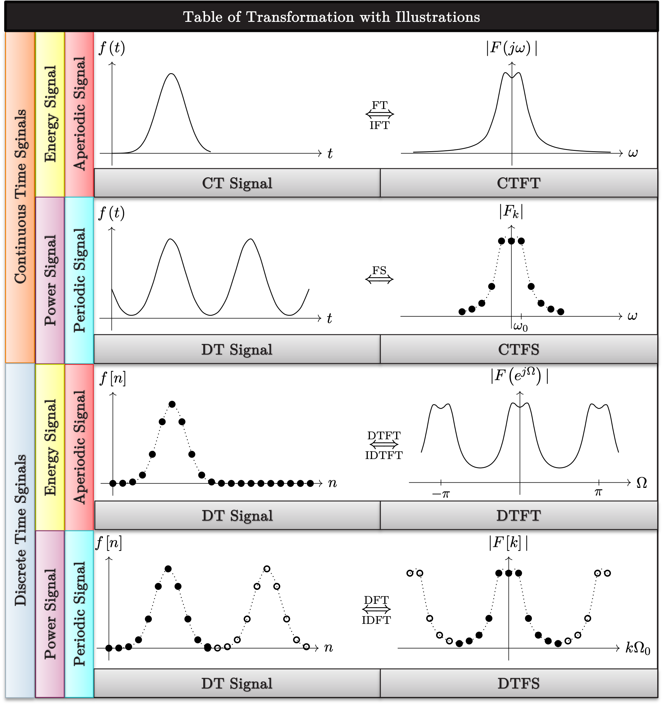
Four-row table of transformations: continuous-time energy/aperiodic signal with CTFT; continuous-time power/periodic signal with CTFS; discrete-time energy/aperiodic sequence with DTFT; discrete-time power/periodic sequence with DTFS/DFT, each row showing the time-domain waveform beside its spectrum
Figure 2.8. The whole lecture on one page. Rows 1–2 are continuous-time (aperiodic, then periodic); rows 3–4 are the discrete-time versions of the same two cases. Read left to right for the time-domain signal, right for its spectrum, and watch the two rules act: going down the table (continuous → discrete time) makes each spectrum periodic; going from row 1 to row 2 (aperiodic → periodic time) makes each spectrum discrete. The last row is the only one where both domains are discrete and finite, which is precisely why it is the only one a computer can store.
Transform
Time domain
Frequency domain
Analysis formula
CTFT
energy signal
continuous,
aperiodic
continuous,
aperiodic
\(\int x(t)e^{-j\Omega t}dt\)
CTFS
power signal
continuous,
periodic \(T_0\)
discrete lines at \(k\Omega_0\),
infinitely many
\(\frac{1}{T_0}\int_{T_0} x(t)e^{-jk\Omega_0 t}dt\)
DTFT
energy sequence
discrete,
aperiodic
continuous,
\(2\pi\)-periodic
\(\sum_n x[n]e^{-j\omega n}\)
DTFS ≡ DFT
power sequence
discrete,
periodic \(N\)
discrete,
periodic: \(N\) lines
\(\sum_{n=0}^{N-1} x[n]e^{-j2\pi kn/N}\)

The fourth class is especially useful for computation. One period contains a finite number of time samples and the spectrum contains the same finite number of coefficients. Both lists fit in memory. This finite representation is the DFT.

Which one do I actually use?

Continuous-time analysis: use the CTFT for aperiodic signals and impulse responses, and the CTFS for periodic signals. Analog filter specifications are written using \(H(j\Omega)\).

Digital filter theory: use the DTFT. FIR and IIR filters are specified through \(H(e^{j\omega})\), while the \(z\)-transform extends the same idea away from the unit circle.

Numerical computation: use the DFT, normally calculated by an FFT. MATLAB spectrum plots, audio analysers and OFDM receivers all use this finite representation.

2.9  The CTFT in use: pairs, and the properties that matter

The first case is an aperiodic continuous-time signal, described by the CTFT in Eq. (2.19). In practice, most transforms are found from a short table of standard pairs together with properties such as scaling, shifting and convolution.

2.9.1  Common CTFT pairs

\(x(t)\)
\(X(\Omega)\)
Remark
\(\delta(t)\)
\(1\)
an impulse contains every frequency equally
\(1\)
\(2\pi\delta(\Omega)\)
the dual: DC is one line at \(\Omega=0\)
\(e^{j\Omega_0t}\)
\(2\pi\delta(\Omega-\Omega_0)\)
one phasor, one spectral line
\(\cos(\Omega_0t)\)
\(\pi[\delta(\Omega-\Omega_0)+\delta(\Omega+\Omega_0)]\)
real and even ⇒ real and even spectrum
\(\sin(\Omega_0t)\)
\(j\pi[\delta(\Omega+\Omega_0)-\delta(\Omega-\Omega_0)]\)
real and odd ⇒ imaginary and odd spectrum
\(e^{-at}u(t)\), \(\Re\{a\}>0\)
\(\dfrac{1}{a+j\Omega}\)
exactly \(H(s)=\frac{1}{s+a}\) at \(s=j\Omega\); a one-pole low-pass
\(\mathrm{rect}(t/T)\)
\(T\,\mathrm{sinc}(\Omega T/2)\)
short in time ⇔ wide in frequency
\(\mathrm{sinc}(t/T)\)
\(2\pi T\,\mathrm{rect}(\Omega T/2)\)
the dual: the ideal brick-wall filter of Lecture 7

Constant signals and pure sinusoids have infinite energy, so their CTFTs are represented by impulses in frequency. Also notice the duality between a rectangular pulse and a sinc: a rectangle in one domain corresponds to a sinc-shaped function in the other. This explains why rectangular windows and ideal rectangular filters produce closely related side-lobe behaviour.

EXAMPLE 2.11 · The rectangular pulse, and why short means wide

Find the CTFT of a single pulse of height \(A\) and width \(\tau\), centred at \(t=0\). Where is its first spectral null?

Solution. Integrate over the pulse only, then collapse the two exponentials with Euler (2.25):

$$\begin{aligned} X(\Omega)&=\int_{-\tau/2}^{\tau/2}\!\!A\,e^{-j\Omega t}dt=\frac{A}{j\Omega}\big(e^{j\Omega\tau/2}-e^{-j\Omega\tau/2}\big)\\[3pt] &=\frac{2A\sin(\Omega\tau/2)}{\Omega}=\boxed{A\tau\,\mathrm{sinc}\!\left(\frac{\Omega\tau}{2}\right)} \end{aligned}$$

The first null is where \(\Omega\tau/2=\pi\), i.e. \(\Omega=2\pi/\tau\). Halve the pulse duration and the spectrum doubles in width: a signal cannot be short in time and narrow in frequency. This is the same trade behind the window choice of Section 2.9.3, behind the DFT's frequency resolution in Problem 2.7, and, run in reverse (Section 2.9.1's duality), behind the fact that an ideal brick-wall filter has an infinitely long sinc impulse response — the central difficulty of FIR design in Lecture 7. Note also that this \(X(\Omega)\) is precisely the dashed envelope in Figure 2.11.a.

2.9.2  Convolution becomes multiplication: this is filtering

This is the property the whole module is built on, and it is Eq. (2.4) again with \(s=j\Omega\):

$$\boxed{\;\begin{aligned} y(t)=x(t)*h(t) &\iff Y(j\Omega)=X(j\Omega)\,H(j\Omega)\\[2pt] y[n]=x[n]*h[n] &\iff Y(e^{j\omega})=X(e^{j\omega})\,H(e^{j\omega}) \end{aligned}\;}$$
(2.29)

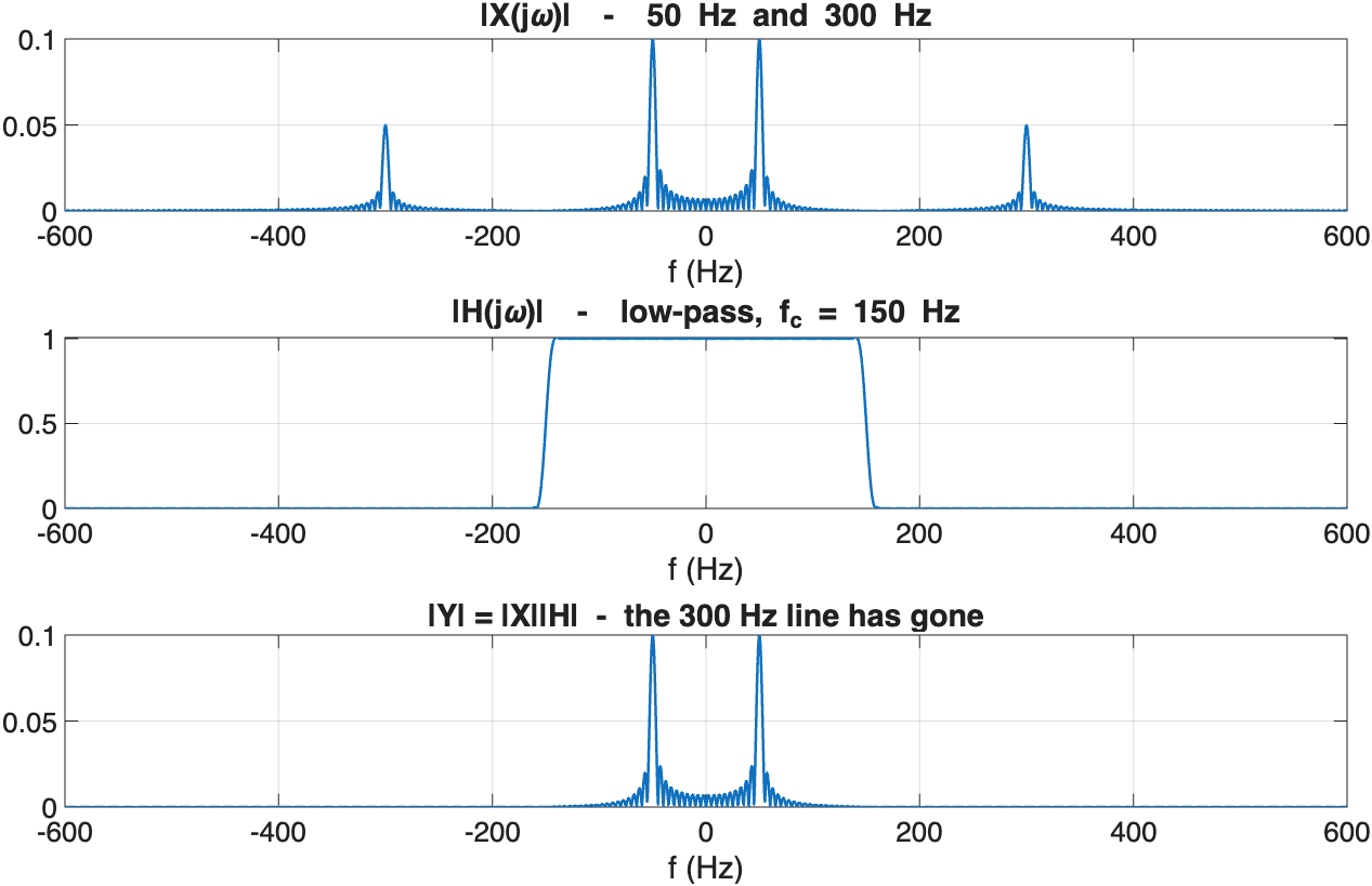
A filter scales each frequency component by \(H(j\Omega)\). For a low-pass filter with \(f_c=150\,\text{Hz}\), the 50 Hz component of a two-tone input remains large, while the 300 Hz component is multiplied by a much smaller value. It is attenuated rather than mathematically erased. Filter design chooses \(H\) so that these frequency-dependent scale factors meet a specification.

2.9.3  Multiplication becomes convolution: windowing and leakage

Run the property the other way and it stops being a convenience and becomes a warning:

$$ z(t)=x(t)\,w(t) \iff Z(j\Omega)=\tfrac{1}{2\pi}\big[X(j\Omega)*W(j\Omega)\big]. $$
(2.30)

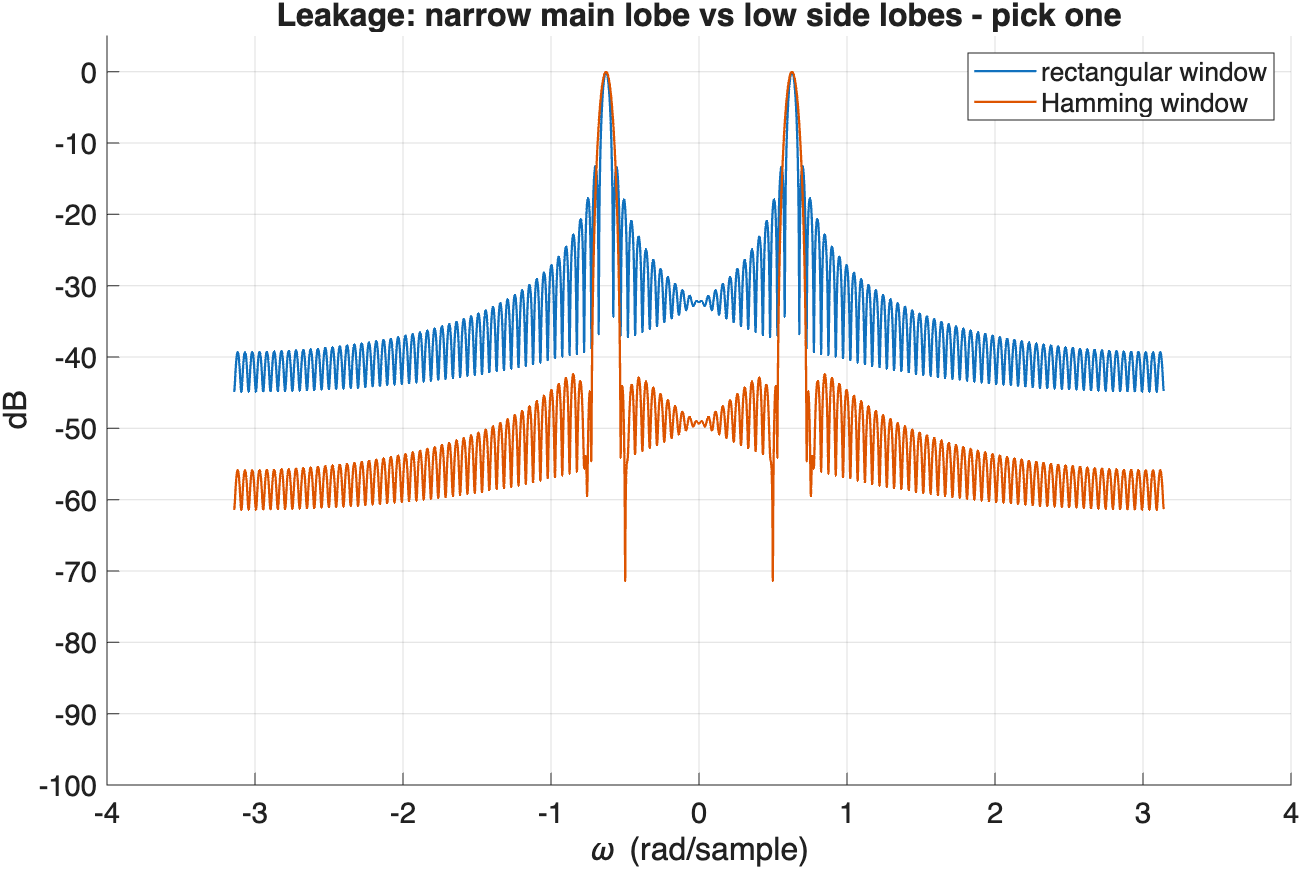
A measurement always has finite duration, which means the true signal has been multiplied by a window. Multiplication in time becomes convolution in frequency, so each ideal spectral line is spread by the window spectrum. This spreading is called spectral leakage; it is a mathematical consequence of finite observation, not a software error.

A rectangular window has a narrow main lobe, which helps separate nearby tones, but high side lobes cause strong leakage. Tapered windows such as Hann, Hamming and Blackman reduce the side lobes but widen the main lobe. Window choice is therefore a trade-off between frequency resolution and leakage.

MATLAB corner

The next script makes Eq. (2.29) and Eq. (2.30) visible in one sitting. Its first half low-pass-filters a two-tone signal purely by multiplying spectra; its second half shows why the window you truncate with decides how badly a clean tone smears.

Goal: show a filter removing a tone purely by spectral multiplication, then show how the truncation window you pick trades main-lobe width against leakage.
L2_7_fixed.m
MATLAB
%% L2_7_fixed.m - Convolution/multiplication demos (non-ASCII spaces removed)
%% Part 1 - Convolution in time IS multiplication in frequency (Eq. 2.29)
fs = 2000; % fine grid, so the FFT approximates the CTFT
t = -0.1 : 1/fs : 0.1;
x = sin(2*pi*50*t) + 0.5*sin(2*pi*300*t);
 
fc = 150; % low-pass cut-off in Hz
h = 2*fc.*sinc(2*fc.*t) .* hann(numel(t))'; % windowed ideal LPF
 
N = 4096; f = (-N/2:N/2-1)*fs/N;
X = fftshift(fft(x,N))/fs;
H = fftshift(fft(h,N))/fs;
Y = X .* H; % <-- the entire point of the section
 
figure('Color','w');
subplot(3,1,1); plot(f,abs(X),'LineWidth',1.2); xlim([-600 600]); grid on;
title('|X(j\Omega)| - 50 Hz and 300 Hz'); xlabel('f (Hz)');
subplot(3,1,2); plot(f,abs(H),'LineWidth',1.2); xlim([-600 600]); grid on;
title('|H(j\Omega)| - low-pass, f_c = 150 Hz'); xlabel('f (Hz)');
subplot(3,1,3); plot(f,abs(Y),'LineWidth',1.2); xlim([-600 600]); grid on;
title('|Y| = |X||H| - the 300 Hz line has gone'); xlabel('f (Hz)');
 
%% Part 2 - Multiplication in time IS convolution in frequency (Eq. 2.30)
% 0.1 cycles/sample over L = 128 samples is 12.8 cycles: NOT a whole
% number, so the assumed periodic extension has a jump -> leakage.
L = 128; Nfft = 4096; n = 0:L-1;
xs = sin(2*pi*0.1*n);
Wr = abs(fftshift(fft(xs .* rectwin(L)', Nfft)));
Wh = abs(fftshift(fft(xs .* hamming(L)', Nfft)));
w = (-Nfft/2:Nfft/2-1)/Nfft*2*pi;
figure('Color','w'); hold on; grid on;
plot(w, 20*log10(Wr/max(Wr)), 'LineWidth', 1.1);
plot(w, 20*log10(Wh/max(Wh)), 'LineWidth', 1.1);
xlabel('\omega (rad/sample)'); ylabel('dB'); ylim([-100 5]);
legend('rectangular window', 'Hamming window');
title('Leakage: narrow main lobe vs low side lobes - pick one');
Three stacked spectra: |X(jw)| showing lines at 50 Hz and 300 Hz, |H(jw)| a low-pass magnitude response with cutoff at 150 Hz, and |Y| showing only the 50 Hz line remaining after multiplication Leakage plot in dB comparing a rectangular window and a Hamming window: the rectangular window has a narrower main lobe but side lobes around -13 dB, the Hamming window has a wider main lobe but side lobes below -40 dB
Figure 2.9. Two MATLAB results, two lessons. On the left, the input contains tones at 50 Hz and 300 Hz. The low-pass filter multiplies each spectral line by the value of \(|H|\) at that frequency. The 50 Hz component remains large, while the 300 Hz component is strongly attenuated; it is not mathematically deleted. On the right, a rectangular window gives a narrower main lobe, so close tones are easier to separate, but its high side lobes spread energy into distant bins. The Hamming window widens the main lobe but greatly reduces that leakage.

2.9.4  A delay is a linear phase ramp

$$\begin{aligned} x(t-t_0)&\iff e^{-j\Omega t_0}X(j\Omega)\\[2pt] x[n-n_0]&\iff e^{-j\omega n_0}X(e^{j\omega}) \end{aligned}$$
(2.31)

A time delay leaves the magnitude unchanged and adds a phase term \(-\Omega t_0\), which is linear in frequency. Conversely, a filter with linear phase delays every frequency component by the same time, so the waveform shape is preserved. Nonlinear phase gives different delays to different components and can distort pulses even when the magnitude response is acceptable.

2.9.5  Parseval: the frequency domain is not a metaphor

One last property makes the spectrum quantitative rather than decorative. Taking inner products through the convolution theorem gives

$$\boxed{\;E=\int_{-\infty}^{\infty}|x(t)|^{2}dt = \frac{1}{2\pi}\int_{-\infty}^{\infty}|X(\Omega)|^{2}d\Omega.\;}$$
(2.32)

Parseval's relation states that the signal energy calculated in time equals the energy calculated in frequency. The transform changes the representation, not the total energy. This allows filter performance to be measured by integrating \(|X(\Omega)|^2\) over passbands or stopbands.

2.10  Frequency-selective filters: the ideal, and why you cannot have it

Because convolution becomes multiplication in frequency, we can design a filter by choosing the shape of \(H(j\Omega)\). Most frequency-selective filters belong to one of four groups: lowpass, highpass, bandpass or bandstop.

lowpassΩ|H| highpassΩ|H| bandpassΩ|H| bandstopΩ|H|
Figure 2.10. The four frequency-selective archetypes, drawn as ideal (brick-wall) magnitude responses. The dashed amber curve on the lowpass panel is what a realizable filter does instead: a finite transition band, ripple, and a stopband that attenuates rather than annihilates.

The ideal lowpass filter is defined by nothing more than an indicator function on frequency, with cutoff \(\Omega_c\):

$$H_{\mathrm{ideal}}(j\Omega) = \begin{cases} 1, & |\Omega| \le \Omega_c \\ 0, & |\Omega| > \Omega_c \end{cases}$$
(2.33)

This ideal response is a useful design target, but it cannot be implemented exactly. Taking its inverse Fourier transform gives

$$h_{\mathrm{ideal}}(t) = \frac{1}{2\pi}\int_{-\Omega_c}^{\Omega_c} e^{j\Omega t}\,d\Omega = \frac{\sin(\Omega_c t)}{\pi t} = \frac{\Omega_c}{\pi}\,\mathrm{sinc}\!\left(\frac{\Omega_c t}{\pi}\right),$$
(2.34)

The result is a sinc impulse response that exists for all time, including \(t<0\). A real-time filter cannot respond before the input arrives, so the ideal filter is non-causal. It is also infinitely long and decays slowly as \(1/t\). Cutting it to a finite length makes implementation possible, but introduces ripple in the frequency response. Lecture 7 shows how window functions control this trade-off.

Ideal

Zero transition width, no ripple, infinite stopband attenuation, zero or linear phase. Non-causal, infinite in duration, unrealisable.

Realizable

Finite transition band \(\Omega_p\to\Omega_s\), passband ripple \(\delta_p\), stopband attenuation \(A_s\), finite order. Every one of these is a number you trade against the others.

A practical filter is therefore specified by four quantities: the passband edge, the stopband edge, the allowed passband ripple and the required stopband attenuation. Lectures 5 and 7 show how to meet these requirements with the lowest reasonable filter order. The brick-wall response remains a reference, not a realizable design.

EXAMPLE 2.12 · How non-causal is the ideal filter?

An ideal lowpass filter has cutoff \(f_c = 1\ \text{kHz}\). Quantify its non-causality: find \(h(t)\) for \(t<0\), and estimate how long a delay would be needed before a truncated version could be built.

Step 1. With \(\Omega_c = 2\pi f_c = 6283\ \text{rad/s}\), Eq. (2.34) gives \(h(t) = \dfrac{\sin(6283\,t)}{\pi t}\). Since \(\sin\) is odd and \(t\) is odd, \(h(-t)=h(t)\): the impulse response is even, so exactly half its energy sits at negative time.

Step 2. Its zero crossings are at \(t = k/(2f_c) = k \times 0.5\ \text{ms}\), so the main lobe spans \(\pm 0.5\ \text{ms}\) and the ripples decay as \(1/t\).

Step 3. To build it, truncate to \(|t| \le T\) and shift right by \(T\), making it causal at the cost of a delay. Keeping ten side lobes means \(T \approx 10 \times 0.5\ \text{ms} = 5\ \text{ms}\), so the filter delays every signal by \(5\ \text{ms}\).

Step 4. The trade is now visible in one place: a sharper cutoff needs a longer \(T\), which is more delay and more coefficients, and truncating at any finite \(T\) reintroduces ripple. Lecture 7 does exactly this calculation with a window in place of the hard cut.

2.11  Rung two: periodic signals and the CT Fourier series

The ordinary CTFT integral does not converge for a periodic signal. Instead, we describe the signal using a Fourier series. If \(x(t)\) repeats every \(T_0\), its frequency components occur only at integer multiples of the fundamental frequency \(\Omega_0=2\pi/T_0\). These frequencies \(k\Omega_0\) are called harmonics, so a sum is sufficient; we do not need an integral over every possible frequency.

$$\boxed{\;\begin{aligned} \text{synthesis:}\quad x(t)&=\sum_{k=-\infty}^{\infty}X_k\,e^{jk\Omega_0 t}\\[3pt] \text{analysis:}\quad X_k&=\frac{1}{T_0}\int_{T_0}x(t)\,e^{-jk\Omega_0 t}\,dt \end{aligned}\;}$$
(2.35)

The analysis formula isolates one harmonic at a time. Multiplying by \(e^{-jk\Omega_0t}\) and integrating over one period makes all other harmonics cancel because they are orthogonal. The complex coefficient \(X_k\) stores both the amplitude and phase of harmonic \(k\). For a real signal, \(X_{-k}=X_k^{*}\), so the magnitude spectrum is even and the phase spectrum is odd.

Parseval reappears too, now measuring power instead of energy, exactly as the energy/power split of Lecture 1 demands:

$$ P=\frac{1}{T_0}\int_{T_0}|x(t)|^{2}dt = \sum_{k=-\infty}^{\infty}|X_k|^{2}. $$
(2.36)

The average power of a periodic signal is the sum of the powers of its harmonics; a sinusoid of amplitude \(A\) has \(P=A^2/2\), split evenly between its two lines at \(\pm\Omega_0\).

2.11.1  The CTFS and the CTFT are not rivals

The CTFS and CTFT are complementary descriptions, not competing methods. Taking the CTFT of the Fourier-series expression term by term, and using \(e^{jk\Omega_0t}\leftrightarrow 2\pi\delta(\Omega-k\Omega_0)\), gives

$$\boxed{\;X(j\Omega)=2\pi\sum_{k=-\infty}^{\infty}X_k\,\delta(\Omega-k\Omega_0).\;}$$
(2.37)

In the generalized sense, the CTFT of a periodic signal is an impulse train. One impulse appears at each harmonic \(k\Omega_0\), weighted by the same coefficient \(X_k\) used in the Fourier series. The two descriptions therefore contain the same information. For calculations, it is usually simpler to list the coefficients \(X_k\) than to write the full impulse spectrum.

CTFS · synthesis

Represents a periodic signal as a sum of harmonics. Use the coefficients \(X_k\) to identify how much of each harmonic is present or to reconstruct the repeating waveform.

CTFT · analysis

Normally gives a continuous spectrum for an aperiodic energy signal. For a periodic signal, it gives the impulse train in Eq. (2.37), carrying the same information as the CTFS coefficients.

2.11.2  The periodic square wave, and a sinc that will come back

Take the standard test case: amplitude \(A\), pulse width \(\tau\), period \(T_0\). Only the pulse contributes to the integral, so

$$\begin{aligned} X_k&=\frac{1}{T_0}\int_{-\tau/2}^{\tau/2} A\,e^{-jk\Omega_0 t}\,dt = \frac{A}{T_0}\cdot\frac{e^{jk\Omega_0\tau/2}-e^{-jk\Omega_0\tau/2}}{jk\Omega_0}\\[4pt] &= \frac{2A\sin(k\Omega_0\tau/2)}{T_0\,k\Omega_0} = \frac{A\tau}{T_0}\,\mathrm{sinc}\!\left(\frac{k\Omega_0\tau}{2}\right) \end{aligned}$$
(2.38)

The middle step is just Euler's formula (2.25) read backwards, which is the third time in this lecture that a messy integral has been rescued by turning exponentials into a sine.
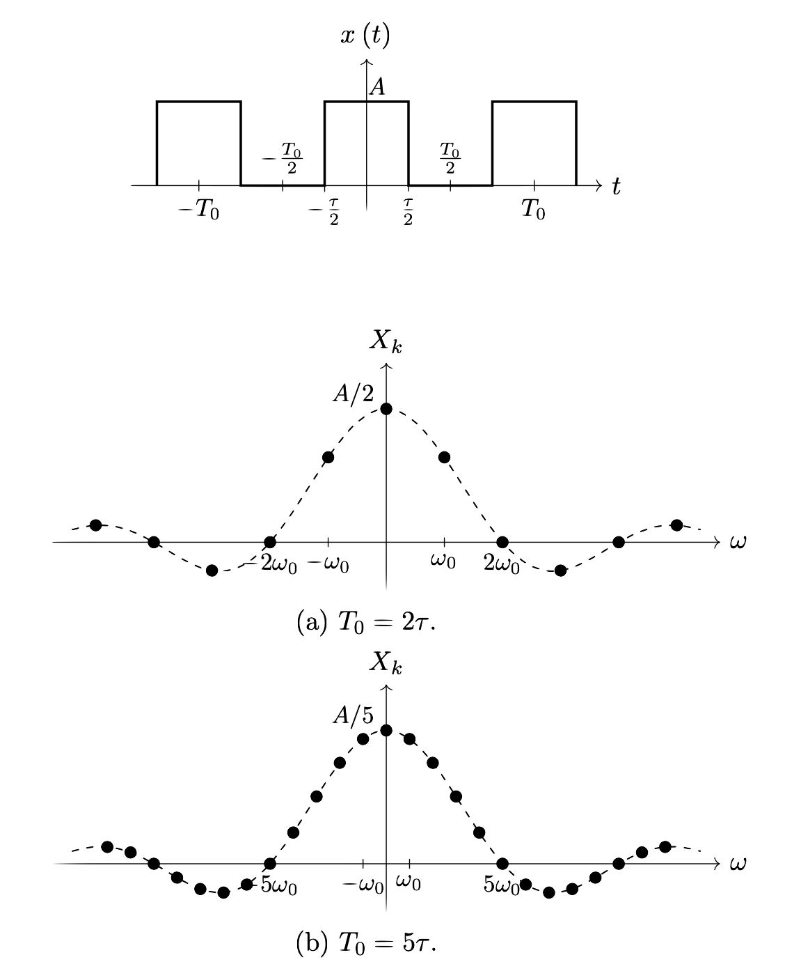
Periodic square wave x(t) of amplitude A, width tau, period T0, with its Fourier coefficients X_k plotted for T0=2 tau and T0=5 tau, both lying on the same sinc envelope but sampled at different densities
Figure 2.11.a. The single most useful picture in this section. Both coefficient plots lie on the same dashed sinc envelope, because the envelope is set by the pulse alone — it is the CTFT of one isolated pulse (Section 2.9.1). Stretching the period from \(T_0=2\tau\) to \(T_0=5\tau\) does not change that curve; it only packs the harmonics more densely along it (and scales them by \(\tau/T_0\)). Let \(T_0\to\infty\) and the lines merge into the continuous CTFT of a single pulse: rung 2 becomes rung 1 in the limit.
EXAMPLE 2.13 · Fourier series of a square wave, with numbers

For the periodic square wave with \(A=1\), \(\tau=1\), \(T_0=4\), find \(X_k\) and check the power against Parseval.

Step 1. Here \(\Omega_0=2\pi/T_0=\pi/2\), so \(k\Omega_0\tau/2=k\pi/4\), and Eq. (2.38) gives

$$X_k=\frac{A\tau}{T_0}\,\mathrm{sinc}\!\left(\frac{k\pi}{4}\right)=\frac{1}{4}\cdot\frac{\sin(k\pi/4)}{k\pi/4}=\frac{\sin(k\pi/4)}{k\pi}.$$

Step 2. Evaluating: \(X_0=0.250\) (which must equal the duty cycle \(\tau/T_0=1/4\), and does), \(X_{\pm1}=0.225\), \(X_{\pm2}=0.159\), \(X_{\pm3}=0.075\), \(X_{\pm4}=0\) (the first null, at \(\Omega=4\Omega_0=2\pi/\tau\), exactly as Example 2.11 predicts), \(X_{\pm5}=-0.045\).

Step 3 · Parseval check. Directly, \(P=\frac{1}{T_0}\int_{T_0}|x|^2dt=\frac{A^2\tau}{T_0}=0.25\). Summing \(|X_k|^2\) out to \(k=\pm7\) gives \(0.2375\), i.e. 95 % of the total power in the first fifteen harmonics — the rest trails off as the sinc envelope decays.

That last number is the practical content of the whole section: a square wave has infinitely many harmonics, but almost all of its power lives in the first few, which is why a band-limited channel can carry a recognisable square pulse at all.

MATLAB corner

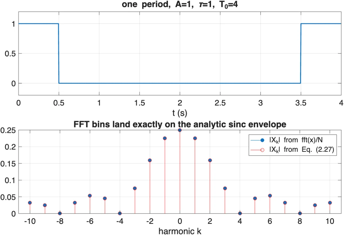
Example 2.13 found the Fourier-series coefficients by integration. Here we sample one period of the same square wave and calculate an FFT. Dividing the FFT by the number of samples gives coefficients that can be compared directly with the analytic values.

Goal: build Example 2.13's square wave, take its FFT, and check the bins against the analytic \(X_k\) of Eq. (2.38) and the power split of Eq. (2.36).
square_wave_fft.m
MATLAB
% square_wave_fft.m - Example 2.13's square wave, checked against the FFT
A = 1; tau = 1; T0 = 4; fs = 200; % Example 2.13's numbers
t = (0:1/fs:T0-1/fs)';
x = A * (mod(t+tau/2, T0) < tau); % one period, pulse centred at t=0
N = numel(x);
 
Xk_fft = fft(x)/N; % DFT/N approximates the CTFS, Eq. (2.47) vs (2.35)
k = (0:N-1)'; k(k>N/2) = k(k>N/2) - N; % centre the harmonic index on 0
w0 = 2*pi/T0;
Xk_analytic = (A*tau/T0) * sinc(k*w0*tau/(2*pi)); % Eq. (2.38)
fprintf('max |FFT - analytic| for |k|<=10: %.2e\n', max(abs(Xk_fft(abs(k)<=10) - Xk_analytic(abs(k)<=10))));
 
P_total = A^2*tau/T0; % Eq. (2.36), direct power
P_partial = @(K) sum(abs(Xk_fft(abs(k)<=K)).^2);
fprintf('power in |k|<=7: %.1f%% of total\n', 100*P_partial(7)/P_total);
 
figure('Color','w');
subplot(2,1,1); plot(t, x, 'LineWidth', 1.6); grid on; ylim([-0.2 1.2]);
title('one period, A=1, \tau=1, T_0=4'); xlabel('t (s)');
 
subplot(2,1,2); stem(k(abs(k)<=10), abs(Xk_fft(abs(k)<=10)), 'filled'); hold on;
stem(k(abs(k)<=10), abs(Xk_analytic(abs(k)<=10)), 'ro'); grid on;
legend('|X_k| from fft(x)/N', '|X_k| from Eq. (2.38)'); xlabel('harmonic k');
title('FFT bins land exactly on the analytic sinc envelope');
Figure 2.11.b — time-domain pulse and FFT bins produced by square_wave_fft.m
Figure 2.11.b. Reading the FFT comparison. The FFT markers lie on the analytic Fourier-series coefficients from Eq. (2.38), including the zeros of the sinc-shaped envelope. This agreement shows that a sampled period contains the same harmonic information as the integral calculation, provided the FFT is scaled by \(1/N\). Summing \(|X_k|^2\) for the 15 lines \(k=-7,\ldots,7\) accounts for about \(95\%\) of the total power. The remaining power is spread over the higher harmonics that form the sharp pulse edges.

This relationship will return in Section 2.14 with time and frequency exchanged. Making a signal periodic in time produces discrete frequency lines. In the opposite direction, sampling a spectrum at discrete frequencies makes the reconstructed time sequence periodic. This is the periodicity assumption built into the DFT.

2.11.3  Gibbs phenomenon: the overshoot that never leaves

Adding more harmonics gives a better square-wave approximation overall, because the total error energy decreases as \(N\) increases. Near each discontinuity, however, a visible overshoot remains.

Each partial sum overshoots the jump, and the overshoot does not shrink. Increasing \(N\) makes the ripple narrower and pushes it closer to the edge, but its height converges to a fixed fraction of the jump:

$$\lim_{N\to\infty}\;\max_t\,\big|x_N(t)\big| = \left(\frac{1}{2}+\frac{1}{\pi}\int_0^{\pi}\frac{\sin u}{u}\,du\right)\Delta \approx 1.0895\,\Delta,$$
(2.39)

The limiting overshoot is approximately \(8.95\%\) of the jump height \(\Delta\) on each side. This is the Gibbs phenomenon. Increasing \(N\) makes the ripple narrower but does not remove its peak height. The ripple energy still tends to zero because it is concentrated into a smaller region.

Why this matters for filter design. Abruptly truncating Fourier coefficients is equivalent to applying a rectangular window, whose sinc-shaped side lobes cause ringing near a jump. The same effect appears when an ideal filter impulse response is cut to a finite length. Lecture 7 uses smoother windows, such as Hamming or Blackman, to reduce the side lobes and therefore reduce the ripple.

gibbs_demo.m
MATLAB
% gibbs_demo.m - partial-sum reconstruction of a square wave, and the
% overshoot that will not go away (Eq. 2.39)
T0 = 1; t = linspace(-1.5*T0, 1.5*T0, 4000);
Ns = [5 15 51 201]; % number of harmonics kept
% odd-harmonic Fourier series of a unit-amplitude square wave
figure; hold on
for N = Ns
x = zeros(size(t));
for k = 1:2:N
x = x + (4/(pi*k)) * sin(2*pi*k*t/T0);
end
plot(t, x, 'LineWidth', 1.0)
end
yline(1, 'k--'); yline(1.0895, 'r:') % ideal level and 8.95% overshoot
legend(compose('N = %d', Ns), 'Location', 'southeast')
xlabel('t / s'); ylabel('partial sum'); grid on
% peak overshoot, measured near the discontinuity at t = 0
for N = Ns
x = zeros(size(t));
for k = 1:2:N, x = x + (4/(pi*k))*sin(2*pi*k*t/T0); end
fprintf('N = %3d peak = %.4f\n', N, max(x));
end
Figure 2.11.c. Interpreting the Gibbs result. Adding more harmonics makes the reconstruction flatter between the discontinuities and confines the oscillations to a narrower region around each jump. However, the largest overshoot does not disappear; it approaches about \(8.95\%\) of the jump height. Increasing \(N\) therefore improves the reconstruction almost everywhere, but it moves the persistent overshoot closer to the discontinuity rather than removing it.
EXAMPLE 2.14 · Does more computation help?

A square wave of amplitude \(\pm 1\) is reconstructed from its first \(N\) harmonics. A colleague reports a peak of \(1.09\) at \(N=51\) and proposes running \(N=5000\) overnight to remove it. What peak will they get, and what would actually work?

Step 1. The jump height is \(\Delta = 2\) (from \(-1\) to \(+1\)), so Eq. (2.39) predicts a peak of \(1.0895 \times 1 = 1.0895\) above the mean — matching the reported \(1.09\).

Step 2. At \(N=5000\) the prediction is the same: \(1.0895\). The limit in Eq. (2.39) does not depend on \(N\). The ripple will be roughly \(100\times\) narrower and invisible at plot resolution, but its height is unchanged, and a peak detector would still report it.

Step 3. What works is changing the truncation, not extending it. Weighting the \(k\)-th coefficient by a taper that goes smoothly to zero at \(k=N\) — Fejér, Hamming, Blackman — removes the overshoot entirely, at the price of a slightly less sharp edge.

Step 4. That trade, ripple against transition sharpness, is the same one Example 2.12 found in the ideal filter, and it is the trade Lecture 7 formalises as the window method.

2.12  Rung three: sampling time, and the DTFT

So far, the signals have been continuous in time. From Lecture 3 onward, most signals are stored as sample arrays, so we need frequency-domain tools for sequences. For an aperiodic sequence \(x[n]\), replace the CTFT integral with a sum and use the discrete-time complex exponential \(e^{-j\omega n}\):

$$\boxed{\;\begin{aligned} X(e^{j\omega})&=\sum_{n=-\infty}^{\infty}x[n]\,e^{-j\omega n}\\[3pt] x[n]&=\frac{1}{2\pi}\int_{-\pi}^{\pi}X(e^{j\omega})\,e^{j\omega n}\,d\omega \end{aligned}\;}$$
(2.40)

This is the Discrete-Time Fourier Transform (DTFT). Like the CTFT, it maps an aperiodic signal to a continuous spectrum. The notation \(X(e^{j\omega})\) reminds us that discrete-time frequency has an important new property: it is periodic.

2.12.1  Why the spectrum repeats every \(2\pi\)

Rule 1 of Section 2.8, read backwards, predicted it: discrete in time \(\Rightarrow\) periodic in frequency. The proof takes one line, and it needs only that \(n\) is an integer:

$$\begin{aligned} e^{-j(\omega+2\pi)n}&=e^{-j\omega n}\underbrace{e^{-j2\pi n}}_{=\,1\ \forall n\in\mathbb{Z}}=e^{-j\omega n}\\[3pt] \Longrightarrow\quad X(e^{j(\omega+2\pi k)})&=X(e^{j\omega}),\qquad k\in\mathbb{Z} \end{aligned}$$
(2.41)

Discrete-time frequency repeats every \(2\pi\). For integer \(n\), \(\cos(\omega n)\) and \(\cos((\omega+2\pi)n)\) produce exactly the same samples. We therefore need only one frequency interval, usually \((-\pi,\pi]\). Frequencies outside it fold back into this interval. In Lecture 3, this folding is called aliasing, and the Nyquist condition is used to prevent different continuous-time frequencies from becoming indistinguishable after sampling.

−3π−2π−π0π shaded: the only interval that carries new information |X(eⁱᵧ)|
Figure 2.12. The DTFT of a five-sample rectangular sequence. The spectrum is continuous in \(\omega\) (rung three's signature) but repeats identically every \(2\pi\), so plotting it outside \((-\pi,\pi]\) adds nothing. Compare the shape with the \(\mathrm{rect}\leftrightarrow\mathrm{sinc}\) pair of Section 2.9.1: a finite pulse gives a sinc-like spectrum in discrete time too (the Dirichlet kernel), which is why truncating data leaks in exactly the way Section 2.9.3 described.

2.12.2  Frequency response, and a hidden Fourier series

Apply Eq. (2.40) to an impulse response and you get the object that the whole second half of the module is written in, the frequency response of an LSI system, which Eq. (2.26) already produced as the eigenvalue:

$$ H(e^{j\omega})=\sum_{n=-\infty}^{\infty}h[n]\,e^{-j\omega n}. $$
(2.42)

Verifying that the inverse in Eq. (2.40) really does recover \(h[n]\) is a one-line application of orthogonality, and it is worth doing because it shows the machinery of Section 2.7.2 working in the discrete world:

$$\begin{aligned} \frac{1}{2\pi}\int_{-\pi}^{\pi}\!\Big[\sum_{k}h[k]e^{-j\omega k}\Big]e^{j\omega n}\,d\omega &= \frac{1}{2\pi}\sum_{k}h[k]\underbrace{\int_{-\pi}^{\pi}\!e^{j\omega(n-k)}\,d\omega}_{=\,0\ (n\neq k),\ =\,2\pi\ (n=k)}\\[3pt] &= h[n] \end{aligned}$$
(2.43)
A connection worth pausing on

Compare Eqs. (2.42)–(2.43) with the Fourier-series pair in Eq. (2.35). Because \(H(e^{j\omega})\) is continuous and \(2\pi\)-periodic in \(\omega\), it has a Fourier series. Equation (2.42) is that series, with the roles of time and frequency exchanged:

CTFS (Section 2.11)
$$x(t)=\sum_k X_k e^{jk\Omega_0 t}$$
$$X_k=\tfrac{1}{T_0}\int_{T_0}x(t)e^{-jk\omega_0t}dt$$
DTFT (this section)
$$H(e^{j\omega})=\sum_n h[n]e^{-j\omega n}$$
$$h[n]=\tfrac{1}{2\pi}\int_{-\pi}^{\pi}H(e^{j\omega})e^{j\omega n}d\omega$$

The key result is that the impulse-response samples \(h[n]\) are the Fourier-series coefficients of the frequency response. This is the basis of the FIR window method in Lecture 7: specify the desired \(H(e^{j\omega})\), find its Fourier coefficients, and use those coefficients as the filter taps.

The familiar Fourier properties still apply in discrete time. Convolution becomes multiplication, windowing causes spectral convolution and leakage, a time delay adds linear phase, and a real sequence has an even magnitude spectrum and an odd phase spectrum: \(X(e^{j\omega})=X^{*}(e^{-j\omega})\).

\(x[n]\)
\(X(e^{j\omega})\)
Remark
\(\delta[n]\)
\(1\)
flat spectrum
\(\delta[n-n_0]\)
\(e^{-j\omega n_0}\)
delay → linear phase, Eq. (2.31)
\(e^{j\omega_0 n}\)
\(2\pi\sum_k\delta(\omega-\omega_0-2\pi k)\)
one line, repeated every \(2\pi\)
\(\cos(\omega_0 n)\)
\(\pi\sum_k\delta(\omega\mp\omega_0-2\pi k)\)
conjugate pair, repeated
\(a^{n}u[n]\), \(|a|<1\)
\(\dfrac{1}{1-ae^{-j\omega}}\)
the workhorse one-pole IIR filter
\(\mathrm{rect}[n/N]\)
\(e^{-j\omega(N-1)/2}\dfrac{\sin(N\omega/2)}{\sin(\omega/2)}\)
Dirichlet kernel; the rectangular window of Figure 2.7.b

2.12.3  When does the DTFT exist? Stability, again

As with the CTFT, the DTFT exists only when its infinite sum converges. For discrete-time systems, the same stability idea appears with a different geometry: the important boundary is now the unit circle rather than the \(j\Omega\)-axis.

Bound the sum term by term. Since \(|e^{-j\omega n}|=1\) for every \(n\) and every \(\omega\), the exponential contributes nothing to convergence:

$$ \big|X(e^{j\omega})\big| \le \sum_{n=-\infty}^{\infty}\big|x[n]\big|\,\underbrace{\big|e^{-j\omega n}\big|}_{=\,1} = \sum_{n=-\infty}^{\infty}\big|x[n]\big|. $$
(2.44)

A sufficient condition for DTFT convergence is that the sequence is absolutely summable. When the sequence is an impulse response, this is exactly the BIBO stability condition introduced in Lecture 1.

$$\boxed{\;\sum_{n=-\infty}^{\infty}|h[n]|<\infty \iff \text{LSI system is BIBO stable} \iff H(e^{j\omega})\ \text{exists.}\;}$$
(2.45)

Lecture 4 expresses this result using the \(z\)-transform, where \(z=re^{j\omega}\). Setting \(r=1\) evaluates the transform on the unit circle and gives the DTFT. Thus, “the ROC contains the unit circle” is the discrete-time counterpart of “the Laplace ROC contains the \(j\Omega\)-axis.”

Continuous time
Discrete time
General transform
Laplace, \(s=\sigma+j\Omega\)
\(z\)-transform, \(z=re^{j\omega}\)
Fourier lives on
the \(j\Omega\)-axis, \(\sigma=0\)
the unit circle, \(r=1\)
Stable (causal) iff
all poles in the left half-plane
all poles inside the unit circle
Convergence test
\(\int|h(t)|\,dt<\infty\)
\(\sum_n|h[n]|<\infty\)
Marginal case
poles on the \(j\Omega\)-axis
poles on the unit circle

Three consequences follow immediately, and they explain things you will otherwise meet as unexplained rules later in the module.

  • FIR filters always have a DTFT. A finite-length \(h[n]\) is a finite sum, which is absolutely summable no matter what the tap values are. This is the precise reason FIR filters are called “unconditionally stable” in Lecture 7 — there is nothing to check.
  • IIR filters must be checked. For \(h[n]=a^{n}u[n]\), \(\sum_n|a|^{n}\) is a geometric series that converges only for \(|a|<1\) — the very condition Example 2.13 needed, and the same statement as “the pole at \(z=a\) lies inside the unit circle”. Lecture 8's IIR designs live or die by it.
  • Some useful sequences fail the test and are admitted anyway. \(u[n]\) and \(\cos(\omega_0 n)\) are not absolutely summable, so strictly they have no DTFT — yet they are in the table of Section 2.12.2. They are admitted through impulses in the frequency domain, exactly the loophole Eq. (2.37) opened for periodic continuous-time signals. The convergence question and the “which rung of the ladder?” question are once again the same question.
EXAMPLE 2.15 · DTFT of a causal exponential sequence

Find the DTFT of \(x[n]=a^{n}u[n]\) with \(|a|<1\), and describe \(|X(e^{j\omega})|\) for \(a=0.7\).

Step 1. The sum is geometric with ratio \(ae^{-j\omega}\), and \(|ae^{-j\omega}|=|a|<1\) guarantees convergence:

$$\begin{aligned} X(e^{j\omega})&=\sum_{n=0}^{\infty}a^{n}e^{-j\omega n}=\sum_{n=0}^{\infty}\big(ae^{-j\omega}\big)^{n}=\boxed{\frac{1}{1-ae^{-j\omega}}}\\[3pt] |X(e^{j\omega})|&=\frac{1}{\sqrt{1-2a\cos\omega+a^{2}}} \end{aligned}$$

Step 2. With \(a=0.7\): \(|X(e^{j0})|=1/(1-a)=3.33\) and \(|X(e^{j\pi})|=1/(1+a)=0.59\), a ratio of \(5.7\) (\(15\,\text{dB}\)) — a gentle low-pass, and exactly the curve plotted in Figure 2.14.a. Note the convergence condition \(|a|<1\) is the discrete-time echo of Section 2.6: it is what puts the pole inside the unit circle, and Lecture 4 will show that the unit circle plays for the \(z\)-transform precisely the role the \(j\Omega\)-axis plays for Laplace.

2.13  Rung four: periodic sequences and the DTFS

The final case is a sequence that is both discrete and periodic: \(x[n+N]=x[n]\). As before, periodicity in time produces a discrete spectrum. The important new feature is that both the time-domain description and the frequency-domain description now contain only \(N\) numbers.

In continuous time there are infinitely many harmonics \(k\Omega_0\), \(k\in\mathbb{Z}\), all distinct. In discrete time they are not distinct. The \(k\)th and the \((k+N)\)th harmonic are the same sequence:

$$ e^{j\frac{2\pi}{N}(k+N)n}=e^{j\frac{2\pi}{N}kn}\,e^{j2\pi n}=e^{j\frac{2\pi}{N}kn}. $$
(2.46)

There are therefore exactly \(N\) distinct harmonics, not infinitely many, and the sum in the synthesis formula is finite. Everything about this rung is finite:

$$\boxed{\;\begin{aligned} x[n]&=\sum_{k=0}^{N-1}X_k\,e^{j\frac{2\pi}{N}kn}\\[3pt] X_k&=\frac{1}{N}\sum_{n=0}^{N-1}x[n]\,e^{-j\frac{2\pi}{N}kn} \end{aligned}\;}$$
(2.47)

This is the Discrete-Time Fourier Series (DTFS): \(N\) input samples produce \(N\) frequency coefficients, with no integrals or infinite limits. A computer can evaluate this finite calculation directly. As in continuous time, the DTFT of a periodic sequence can also be written as an impulse train at the harmonic frequencies, weighted by the DTFS coefficients.

$$ X(e^{j\omega})=2\pi\sum_{k=0}^{N-1}X_k\,\delta\!\left(\omega-\tfrac{2\pi}{N}k\right). $$
(2.48)
DTFT
DTFS
Signal
aperiodic, infinite length
periodic, period \(N\)
Spectrum
continuous, \(2\pi\)-periodic
\(N\) discrete coefficients
Form
infinite sum / integral
finite sum of \(N\) harmonics
CT analogue
CTFT
CTFS

2.14  The DFT and the FFT: the only one a computer can run

In practice, we usually have a finite block of \(N\) samples. The DTFT is continuous in frequency, so a computer cannot store every value, while the DTFS assumes that the sequence is periodic. The DFT connects these two ideas by treating the available block as one period of a repeating sequence.

The Discrete Fourier Transform (DFT) is what you get by making two decisions, each of which is Rule 1 applied deliberately rather than accidentally:

  1. Truncate in time. Keep \(N\) samples and set the rest to zero, i.e. multiply by a rectangular window (Section 2.9.3, with everything that implies about leakage).
  2. Sample in frequency. Evaluate the DTFT only at \(N\) equally spaced points \(\omega_k=2\pi k/N\), \(k=0,\ldots,N-1\).
$$\boxed{\;\begin{aligned} X[k]&=X(e^{j\omega})\big|_{\omega=2\pi k/N}=\sum_{n=0}^{N-1}x[n]\,e^{-j\frac{2\pi}{N}kn}\\[3pt] x[n]&=\frac{1}{N}\sum_{k=0}^{N-1}X[k]\,e^{j\frac{2\pi}{N}kn} \end{aligned}\;}$$
(2.49)

Apart from the placement of the factor \(1/N\), this is the same formula as the DTFS in Eq. (2.47). The DFT is therefore not a separate fifth transform. It is the DTFS applied to one finite block, with a name that emphasizes its computational use.

EXAMPLE 2.16 · A four-point DFT by hand

Compute the 4-point DFT of \(x=[1,\,1,\,0,\,0]\), and verify conjugate symmetry and Parseval.

Step 1. With \(N=4\), only \(n=0,1\) contribute, so Eq. (2.47) reduces to \(X[k]=1+e^{-j\pi k/2}\):

$$X[0]=2,\quad X[1]=1-j,\quad X[2]=0,\quad X[3]=1+j.$$

Step 2. Magnitudes \(|X|=[2,\ \sqrt2,\ 0,\ \sqrt2]\), phases \([0,\ -45^\circ,\ -,\ +45^\circ]\).

Step 3 · Symmetry. \(X[3]=X[1]^{*}\), as a real input requires (Problem 2.6): the second half of the spectrum carries no new information.

Step 4 · Parseval. \(\sum_n|x[n]|^2=2\) and \(\frac{1}{N}\sum_k|X[k]|^2=\frac{1}{4}(4+2+0+2)=2\). Energy is conserved, exactly as Eq. (2.32) promised in continuous time.

|X(eⁱᵧ)| continuous DTFT N = 8 DFT bins X[k] −π0π the DFT sees the spectrum only where the red stems stand
Figure 2.14.a. The DFT is the DTFT, sampled. The grey curve is the true, continuous \(|X(e^{j\omega})|\); the red stems are the \(N=8\) numbers a computer actually returns. Increasing \(N\) (by taking more data, or by zero-padding) moves the stems closer together and shows more of the curve — but the curve itself is fixed by the data you have, so zero-padding interpolates the picture, it does not add resolution. This is Figure 2.7.c with time and frequency exchanged.
What the DFT quietly assumes, and what it costs you

The inverse DFT reconstructs one period of an \(N\)-periodic sequence. In other words, the DFT assumes that the data block repeats forever, so the sample after the last one is the first sample again.

This assumption has two practical consequences. If the two ends do not join smoothly, the periodic extension contains a discontinuity and energy spreads into nearby bins; this is spectral leakage. Also, multiplying two DFTs produces circular convolution, in which the end of the result wraps to the beginning. Windowing reduces leakage, while the overlap-add and overlap-save methods in Lecture 7 recover linear convolution.

These behaviours are not numerical errors; they follow directly from the DFT's periodic model.

Written out, Eq. (2.47) is a matrix–vector product with \([\mathbf{W}]_{k,n}=e^{-j2\pi kn/N}\), and the inverse is (up to \(1/N\)) its conjugate transpose — the DFT matrix is unitary, which is Parseval's theorem in linear-algebra clothing:

$$ \mathbf{X}=\mathbf{W}\mathbf{x}, \qquad \mathbf{x}=\tfrac{1}{N}\mathbf{W}^{H}\mathbf{X}. $$
(2.50)
Left: original sequence x[n] with IFFT reconstruction and DTFS synthesis overlaid, agreeing to 1e-15; right: the DTFS coefficient magnitudes, showing four nonzero lines
Figure 2.14.b. Eq. (2.47) and Eq. (2.49) are the same computation, checked numerically. The DTFS synthesis and the IFFT reconstruct the original sequence to within \(\sim\!10^{-15}\), i.e. to machine precision: the disagreement is rounding, not mathematics. The coefficients on the right show the conjugate-symmetric pairs a real sequence must have, \(X_k\) and \(X_{N-k}\) matched in magnitude (Problem 2.6).
MATLAB corner

The claim of Section 2.14, that \(X[k]=X(e^{j\omega})|_{\omega=2\pi k/N}\), is easy to state and easier to believe once plotted. This script evaluates Eq. (2.40) on a dense grid by brute force and drops the \(N\) FFT bins on top of it — reproducing Figure 2.14.a from scratch.

Goal: overlay the DFT bins on the dense DTFT curve to confirm the DFT samples it exactly, and show what zero-padding does (and doesn't) add.
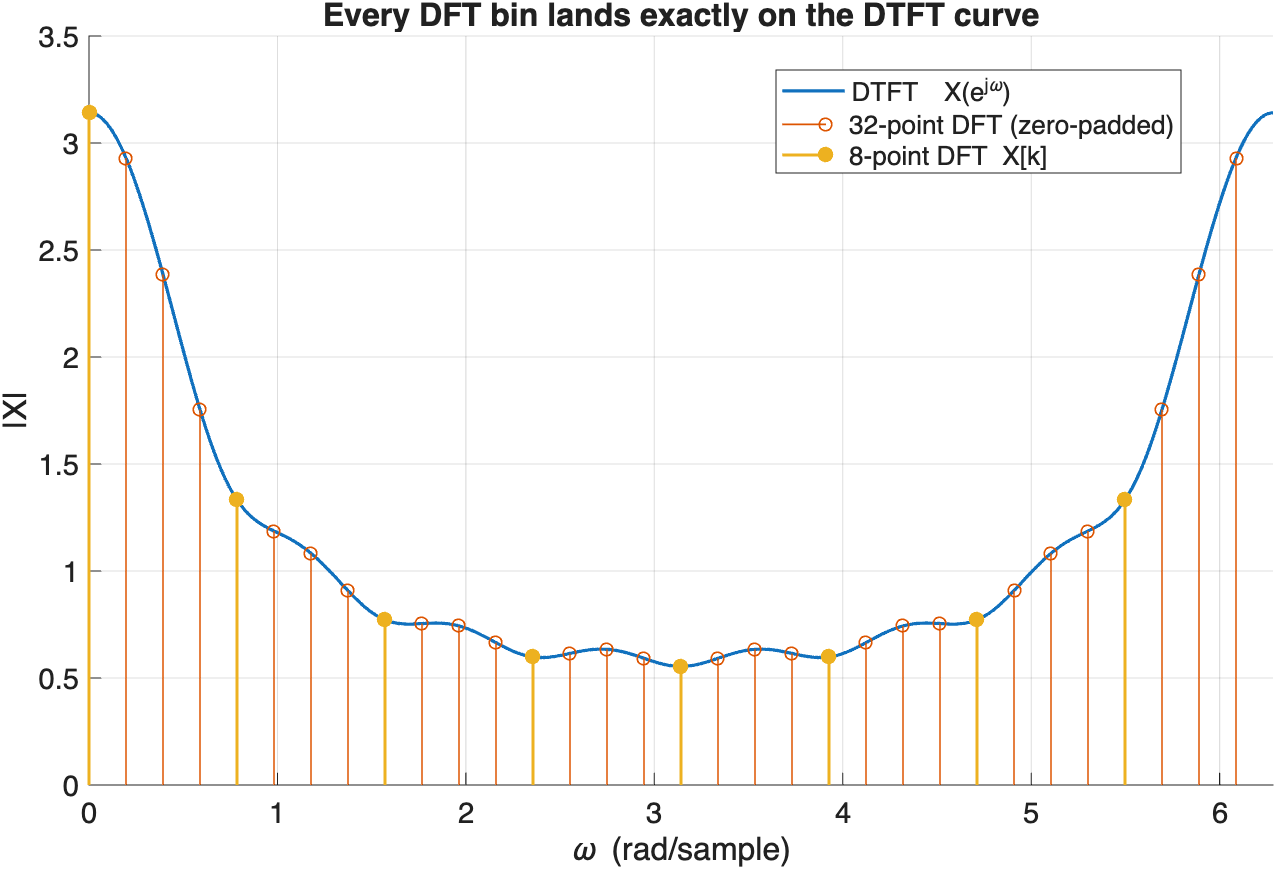
dtft_vs_dft.m
MATLAB
%% The DFT is the DTFT, sampled at N points (Eq. 2.47, Fig. 2.14.b)
a = 0.7; N = 8; Ndense = 2048;
n = 0:N-1;
x = a.^n; % one block of a^n u[n]
% "The DTFT": evaluate the analysis sum on a very fine grid of omega.
wd = linspace(0, 2*pi, Ndense);
Xd = zeros(size(wd));
for k = 1:N
Xd = Xd + x(k)*exp(-1j*wd*n(k));
end
% "The DFT": the same sum, at only N frequencies. fft() does it fast.
Xk = fft(x);
wk = 2*pi*(0:N-1)/N;
% Zero-padding to 4N: MORE points on the SAME curve, not more resolution.
X4 = fft(x, 4*N);
w4 = 2*pi*(0:4*N-1)/(4*N);
figure('Color','w'); hold on; grid on;
plot(wd, abs(Xd), 'LineWidth', 1.6);
stem(w4, abs(X4), 'LineWidth', 0.8);
stem(wk, abs(Xk), 'filled', 'LineWidth', 1.4);
xlabel('\omega (rad/sample)'); ylabel('|X|'); xlim([0 2*pi]);
legend('DTFT X(e^{j\omega})', '32-point DFT (zero-padded)', '8-point DFT X[k]');
title('Every DFT bin lands exactly on the DTFT curve');
% Numerical check: each bin equals the DTFT at that frequency.
Xexact = arrayfun(@(w) sum(x .* exp(-1j*w*n)), wk);
fprintf('max |X[k] - X(e^{j 2 pi k/N})| = %.3e\n', max(abs(Xk - Xexact)));
% -> ~1e-15: they are the same numbers, to machine precision.
Plot showing the continuous DTFT curve of a 0.7^n sequence in blue, overlaid with a 32-point zero-padded DFT as open orange stems and the 8-point DFT as filled yellow stems, all landing exactly on the DTFT curve
Figure 2.14.c. What zero-padding changes. The 8-point DFT gives eight samples of the same continuous DTFT curve. Appending zeros and taking a 32-point DFT gives more closely spaced samples, so the plotted spectrum looks smoother and the peak location can be read more easily. Both sets of markers still lie on the original DTFT. The ability to separate nearby frequencies is fixed by the length of the non-zero data record, so zero-padding improves display sampling but does not create new frequency resolution.

2.14.1  The FFT: same answer, vastly less work

Direct evaluation of an \(N\)-point DFT needs roughly \(N^2\) complex multiplications. For \(N=1024\), that is about one million operations. The Fast Fourier Transform (FFT) computes exactly the same DFT values more efficiently by reusing repeated calculations. The first step is to split the sum into even- and odd-indexed samples:

$$\begin{aligned} X[k]=\underbrace{\sum_{n=0}^{N/2-1}x[2n]\,e^{-j\frac{2\pi kn}{N/2}}}_{\text{an }N/2\text{-point DFT}} \;+\; e^{-j\frac{2\pi k}{N}}\underbrace{\sum_{n=0}^{N/2-1}x[2n{+}1]\,e^{-j\frac{2\pi kn}{N/2}}}_{\text{another }N/2\text{-point DFT}} \end{aligned}$$
(2.51)

The \(N\)-point calculation is now two \(N/2\)-point DFTs plus a set of combining operations. Repeating this split gives a computational cost of order \(N\log_2N\), instead of \(N^2\). The saving grows rapidly with data length:

N = 1024
\(N^2\approx 1.0\times10^{6}\)
\(N\log_2 N\approx 1.0\times10^{4}\)
100× faster
N = 65 536
\(N^2\approx 4.3\times10^{9}\)
\(N\log_2 N\approx 1.0\times10^{6}\)
4 000× faster
N = 1 048 576
\(N^2\approx 1.1\times10^{12}\)
\(N\log_2 N\approx 2.1\times10^{7}\)
52 000× faster

This efficiency makes the FFT practical for real-time processing. Spectrum analysers, OFDM systems such as Wi-Fi and mobile communications, long FIR filtering, and many audio and image codecs all use FFT algorithms to evaluate DFTs repeatedly.

The ladder in seven lines
LT
Damping allowed. Stability, transients, transfer functions. Lecture 5 designs analog filters here.
CTFT
\(\sigma=0\). Continuous spectrum of an energy signal. Where \(|H(j\Omega)|\) lives.
CTFS
Periodic time ⇒ discrete spectrum. The repair for power signals; harmonics of \(\Omega_0\).
DTFT
Discrete time ⇒ \(2\pi\)-periodic spectrum. Where every digital filter is specified.
DTFS
Discrete and periodic ⇒ \(N\) coefficients. Everything finite at last.
DFT
The DTFS of one block, with the periodicity assumed rather than given. What a computer computes.
FFT
Not a transform. The \(\mathcal{O}(N\log N)\) algorithm that makes the DFT practical.

?Problems with solutions

Work each one before reading the solution.

PROBLEM 2.1

Given \(H(s) = \dfrac{s+2}{s^2+2s+5}\): find its poles, classify its stability, and find \(h(t)\).

Solution. Complete the square: \(s^2+2s+5=(s+1)^2+4\), so poles are \(s=-1\pm j2\); both have \(\Re\{s\}=-1<0\), so \(H(s)\) is stable. Write the numerator as \(s+2=(s+1)+1\):

$$H(s) = \frac{s+1}{(s+1)^2+4} + \frac{1}{(s+1)^2+4} = \frac{s+1}{(s+1)^2+4} + \tfrac12\cdot\frac{2}{(s+1)^2+4},$$

matching \(\alpha=1,\beta=2\) with \(A=1\), \(C=\tfrac12\):

$$\boxed{h(t) = e^{-t}\Big[\cos(2t) + \tfrac12\sin(2t)\Big]u(t).}$$
PROBLEM 2.2

A system has \(H(s)=\dfrac{1}{s+3}\). Write down \(H(j\Omega)\), its magnitude and phase, and find the frequency at which the output power is halved.

Solution. The single pole is at \(s=-3\), safely in the left half-plane, so the ROC contains the \(j\Omega\)-axis and Eq. (2.19) may be applied by substitution:

$$H(j\Omega)=\frac{1}{3+j\Omega},\quad |H(j\Omega)|=\frac{1}{\sqrt{9+\Omega^{2}}},\quad \angle H(j\Omega)=-\arctan\frac{\Omega}{3}$$

Half power means \(|H|^{2}\) drops to half its DC value \(|H(0)|^{2}=1/9\), i.e. \(|H|=\frac{1}{3\sqrt2}\):

$$\frac{1}{\sqrt{9+\Omega^{2}}}=\frac{1}{3\sqrt2}\ \Longrightarrow\ 9+\Omega^{2}=18\ \Longrightarrow\ \boxed{\Omega_{-3\text{dB}}=3\ \text{rad/s}.}$$

The corner frequency equals the pole magnitude — the general first-order result, and the reason a pole–zero plot doubles as a rough sketch of the magnitude response. The impulse response is \(h(t)=e^{-3t}u(t)\), matching Example 2.10 with \(a=3\).

PROBLEM 2.3

A rectangular window of length \(L\) has DTFT \(W(e^{j\omega})=e^{-j\omega(L-1)/2}\dfrac{\sin(L\omega/2)}{\sin(\omega/2)}\). Find its main-lobe width. Does increasing \(L\) reduce the side lobes?

Solution. The numerator vanishes when \(L\omega/2=\pm\pi\), i.e. at \(\omega=\pm2\pi/L\), so the main lobe runs from \(-2\pi/L\) to \(+2\pi/L\):

$$\boxed{\Delta\omega_{\text{main}}=\frac{4\pi}{L}.}$$

Doubling \(L\) halves the main-lobe width, so a longer record really does resolve two close tones better — the discrete-time echo of Example 2.11's time–bandwidth trade.

But no, the side lobes do not improve. The first side lobe of a rectangular window sits about \(13\,\text{dB}\) below the peak whatever \(L\) is: increasing \(L\) squeezes the whole pattern horizontally without lowering it. Side-lobe height is a property of the window's shape, not its length, which is why leakage is fought with tapering rather than with more data (Hamming: \(\approx-41\,\text{dB}\) side lobes, at the price of a main lobe twice as wide, \(8\pi/L\)). This single trade-off governs the whole window method of FIR design in Lecture 7.

PROBLEM 2.4

For \(x(t)=A\cos(\Omega_0t)\): explain why the CTFT integral fails, give the CTFS coefficients, verify the power with Parseval, and recover the generalised CTFT from Eq. (2.37).

Why it fails. A cosine never decays, so \(\int|x(t)|dt=\infty\) and \(E=\infty\) (Eq. 2.21). Without the damping factor \(e^{-\sigma t}\) that the Laplace kernel provided, the integral has nothing to make it converge: this is a power signal, and the CTFT is a tool for energy signals.

CTFS. No integration is needed — Euler's formula (2.25) already is the Fourier series, with \(T_0=2\pi/\Omega_0\):

$$\begin{aligned} A\cos(\Omega_0t)&=\tfrac{A}{2}e^{j\Omega_0t}+\tfrac{A}{2}e^{-j\Omega_0t}\\[2pt] &\Longrightarrow\ \boxed{X_{1}=X_{-1}=\tfrac{A}{2},\ \ X_k=0\text{ otherwise}} \end{aligned}$$

Parseval (2.36). \(\sum_k|X_k|^2=\left(\tfrac{A}{2}\right)^2+\left(\tfrac{A}{2}\right)^2=\tfrac{A^2}{2}\), which is the familiar average power of a sinusoid — and it confirms the “negative frequency” line is carrying real, physical half of the power, not a bookkeeping artefact.

Generalised CTFT. Feeding those two coefficients into Eq. (2.37): \(X(\Omega)=2\pi\big[\tfrac{A}{2}\delta(\Omega-\Omega_0)+\tfrac{A}{2}\delta(\Omega+\Omega_0)\big]=A\pi\big[\delta(\Omega-\Omega_0)+\delta(\Omega+\Omega_0)\big]\), exactly the pair tabulated in Section 2.9.1. The transform that “failed” agrees perfectly once impulses are allowed.

PROBLEM 2.5

Show that \(\cos(\omega n)\) and \(\cos\big((\omega+2\pi)n\big)\) are the same sequence, and that \(\cos(\Omega_0 t)\) and \(\cos\big((\Omega_0+2\pi)t\big)\) are not the same signal. What does the difference imply about discrete-time frequency?

Solution. In discrete time the index \(n\) is an integer, so the extra term \(2\pi n\) is always a whole number of revolutions:

$$\cos\big((\omega+2\pi)n\big)=\cos(\omega n+2\pi n)=\cos(\omega n)\quad\forall n\in\mathbb{Z}.$$

In continuous time \(t\) is real, \(2\pi t\) is generally not a whole number of revolutions, and the two cosines differ everywhere except at integer \(t\).

Implication. Discrete-time frequency does not live on a line, it lives on a circle of circumference \(2\pi\). Every distinguishable DT frequency fits in \((-\pi,\pi]\); anything outside is an alias of something inside. Hence the DTFT is \(2\pi\)-periodic (Eq. 2.41), hence \(\omega=\pi\) is the fastest possible oscillation (alternating \(+1,-1,+1,\ldots\)), and hence sampling above twice the highest signal frequency — Nyquist, Lecture 3 — is exactly the condition that stops distinct continuous-time frequencies from colliding on that circle.

PROBLEM 2.6*

Show that the \(N\)-point DFT of a real sequence satisfies \(X[N-k]=X^{*}[k]\). How many independent real numbers does the spectrum contain, and why must the answer be \(N\)? (* optional)

Proof. Substitute \(N-k\) into Eq. (2.49) and use \(e^{-j2\pi n}=1\) for integer \(n\):

$$\begin{aligned} X[N-k]&=\sum_{n=0}^{N-1}x[n]e^{-j\frac{2\pi}{N}(N-k)n}=\sum_{n=0}^{N-1}x[n]\underbrace{e^{-j2\pi n}}_{=1}e^{j\frac{2\pi}{N}kn}\\[3pt] &=\sum_{n=0}^{N-1}x[n]e^{j\frac{2\pi}{N}kn}=X^{*}[k], \end{aligned}$$

where the last step needs \(x[n]=x^{*}[n]\), i.e. \(x\) real. (This is Eq. (2.20)'s conjugate symmetry, now on a finite grid.)

Counting. Bins \(k\) and \(N-k\) are redundant, so only \(k=0,\ldots,N/2\) need be stored: that is \(N/2+1\) complex numbers. But two of them are forced to be real — \(X[0]=\sum_n x[n]\) and \(X[N/2]=\sum_n(-1)^n x[n]\) are both sums of real numbers. So the count of independent real values is

$$\underbrace{2}_{X[0],\,X[N/2]}+\underbrace{2\left(\tfrac{N}{2}-1\right)}_{\text{the complex bins}}=N.$$

It had to be \(N\): the DFT is an invertible map (Eq. 2.50), so it can neither create nor destroy degrees of freedom — \(N\) real samples in, \(N\) real numbers out. Practically, this is why real-input FFT routines return only \(N/2+1\) bins and run about twice as fast, and why every spectrum plot you have seen of a real signal shows only the positive half.

PROBLEM 2.7

You take \(N=8192\) samples at \(f_s=8\,\text{kHz}\) and compute an \(N\)-point DFT. (a) What is the frequency spacing between bins? (b) Where does a \(1000\,\text{Hz}\) tone land? (c) What changes if the tone is at \(1000.5\,\text{Hz}\)? (d) What can you do about it?

(a) The block spans \(N/f_s=1.024\,\text{s}\), and the \(N\) bins divide \(f_s\) evenly:

$$\Delta f=\frac{f_s}{N}=\frac{8000}{8192}=0.9766\ \text{Hz}.$$

(b) \(k=1000/0.9766=1024\) exactly. An integer, which is the good case: the tone completes precisely \(1024\) whole cycles inside the block, so the periodic extension the DFT assumes (Section 2.14) joins up seamlessly, and all the energy appears in bin \(1024\) alone.

(c) \(k=1000.5/0.9766=1024.51\), halfway between bins. The tone now ends mid-cycle, the assumed periodic extension has a step discontinuity that the signal never contained, and its energy sprays across every bin — leakage. Worse, the true peak falls between the two sampling points of Figure 2.11.a, so the measured amplitude reads low by up to \(3.9\,\text{dB}\) (“scalloping loss”).

(d) You cannot make it vanish; you choose which price to pay. Applying a tapered window (Hann, Hamming) before the FFT drops the side lobes by \(30\,\text{dB}\) or more at the cost of a wider peak. Taking a longer record shrinks \(\Delta f\) and improves genuine resolution. Zero-padding does neither: it adds bins between the existing ones (the extra stems in dtft_vs_dft.m), which interpolates the picture and improves the peak reading, but the underlying DTFT is fixed by the data you actually collected.

Summary and key formulas

The reference sheet below: the Laplace results, the four transform pairs in the order the map puts them, and the properties that get used every day.

Laplace transfer function · Eq. (2.5)
$$H(s)=\frac{Y(s)}{X(s)}=K\frac{\prod_k(s-z_k)}{\prod_\ell(s-p_\ell)}$$
Distinct-pole partial fractions · Eq. (2.12)
$$F(s)=\sum_k\frac{A_k}{s-p_k} \leftrightarrow \sum_k A_ke^{p_kt}u(t)$$
Stability and the CTFT · Eq. (2.16), (2.19)
$$\text{BIBO}\iff\Re\{p_k\}<0\ \forall k \;\Rightarrow\; H(\Omega)=H(s)|_{s=j\Omega}$$
Eigenfunction property · Eq. (2.27)
$$e^{j\Omega t}\ \longmapsto\ H(j\Omega)\,e^{j\Omega t}$$
Convolution → multiplication · Eq. (2.29)
$$x*h \ \longleftrightarrow\ X(j\Omega)H(j\Omega)$$
Parseval · Eq. (2.32), (2.36)
$$E=\tfrac{1}{2\pi}\!\int\!|X(\Omega)|^2d\Omega,\quad P=\sum_k|X_k|^2$$
The four rungs · Sections 2.9–2.11
CTFT · CT, aperiodic · Eq. (2.19)
$$X(\Omega)=\int_{-\infty}^{\infty}\!x(t)e^{-j\Omega t}dt$$

Continuous, aperiodic spectrum.

CTFS · CT, periodic · Eq. (2.35)
$$X_k=\tfrac{1}{T_0}\!\int_{T_0}\!x(t)e^{-jk\Omega_0t}dt$$

Discrete lines at \(k\Omega_0\), infinitely many.

DTFT · DT, aperiodic · Eq. (2.40)
$$X(e^{j\omega})=\sum_{n}x[n]e^{-j\omega n}$$

Continuous, \(2\pi\)-periodic spectrum.

DTFS ≡ DFT · DT, periodic · Eq. (2.47), (2.49)
$$X[k]=\sum_{n=0}^{N-1}x[n]e^{-j\frac{2\pi}{N}kn}$$

\(N\) lines. The only computable rung; run it with an FFT.

  • The Laplace transform turns an LCCDE, and convolution itself, into algebra: \(H(s)=Y(s)/X(s)\), a ratio of polynomials whose roots are the system's poles and zeros; partial fractions invert it term by term, one exponential or damped sinusoid per pole.
  • A causal system is stable exactly when every pole lies in the open left-half \(s\)-plane; only then does the ROC contain the \(j\Omega\)-axis, and only then does \(H(j\Omega)=H(s)|_{s=j\Omega}\), the CTFT, exist. Stability and the existence of a frequency response are one statement.
  • Fourier analysis is written in complex exponentials for one reason: they are the eigenfunctions of every LTI/LSI system (Eq. 2.27), so convolution collapses into a multiplication per frequency. Orthogonality then makes each coefficient readable by a single independent integral, and Euler's formula packs amplitude and phase into one number.
  • There are not many transforms — there are exactly four signal classes (CT or DT \(\times\) aperiodic or periodic) and one transform each. Two rules fix every spectrum's shape: periodic in one domain ⇔ discrete in the other, and aperiodic ⇔ continuous.
  • Doing both discretisations at once leaves the DTFS, the one rung with no infinity in it. Renamed for computation it is the DFT, whose price is an assumed periodic extension (hence leakage and circular convolution), and the FFT evaluates it in \(\mathcal{O}(N\log N)\) instead of \(\mathcal{O}(N^2)\).
  • Three properties do most of the daily work: convolution → multiplication (this is filtering), multiplication → convolution (this is windowing, and leakage), and a delay → a linear phase ramp (this is why linear-phase FIR filters exist).
  • Next, in Lecture 3: sampling, quantization and reconstruction — where the \(2\pi\)-periodicity of Eq. (2.41) turns into the Nyquist criterion, and where the passage from \(x(t)\) to \(x[n]\) that this lecture assumed is finally justified.